Next: Step 1: The calculations Up: Electric transport calculations Previous: Electric transport calculations Contents Index
Electronic transport properties of molecules, nano-wires, and bulks such as superlattice structures can be calculated based on a non-equilibrium Green function (NEGF) method within the collinear and non-collinear DFT methods. The features and capabilities are listed below:
The details of the implementation can be found in Ref. [58]. First the usage of the functionalities for the collinear case is explained in the following subsections. After then, the non-collinear case will be discussed.
System we consider
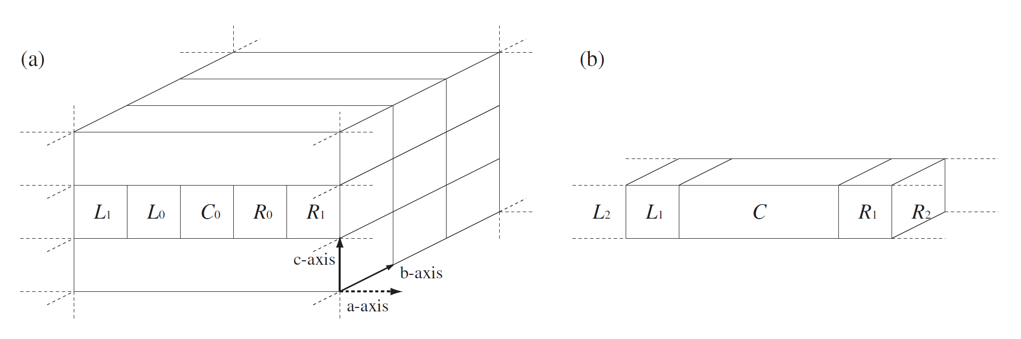
In the current implementation of OpenMX Ver. 3.8, a system shown in Fig. 31(a) is treated
by the NEGF method. The system consists of a central region connected with
infinite left and right leads, and the two dimensional periodicity spreads
over the bc-plane. Considering the two dimensional periodicity, the
system can be cast into a one-dimensional problem depending on
the Bloch wave vector ![]() shown in Fig. 31(b).
Also, the Green function of the region
shown in Fig. 31(b).
Also, the Green function of the region
![]() is self-consistently
determined in order to take account of relaxation of electronic structure around
the interface between the central region
is self-consistently
determined in order to take account of relaxation of electronic structure around
the interface between the central region ![]() and the region
and the region ![]() .
It should be noted that the electronic transport is assumed to be along
the a-axis in the current implementation. Thus, users have to keep in mind
the specification when the geometrical structure is constructed.
See also the subsection 'Step 1: The calculations for leads'.
.
It should be noted that the electronic transport is assumed to be along
the a-axis in the current implementation. Thus, users have to keep in mind
the specification when the geometrical structure is constructed.
See also the subsection 'Step 1: The calculations for leads'.
 |
Computational flow
The NEGF calculation is performed by the following three steps:
Step 1 ![]() Step 2
Step 2 ![]() Step 3
Step 3
Each step consists of
The band structure calculations are performed for the left and right leads using a program code 'openmx'. The calculated results will be used to represent the Hamiltonian of the leads in the NEGF calculation of the step 2.
The NEGF calculation is performed for the structure shown in Fig. 31 under zero or a finite bias voltage using a program code 'openmx', where the result in the step 1 is used for the construction of the leads.
By making use of the result of the step 2, the transmission, charge/spin current density, and the eigenchannel are calculated by a program code 'openmx'.
An example: carbon chain
As a first trial, let us illustrate the three steps by employing a carbon chain. Before going to the illustration,
Step 1
%./openmx Lead-Chain.dat | tee lead-chain.std
Step 2
%./openmx NEGF-Chain.dat | tee negf-chain.std
Step 3
openmx starts step 3 immediately after it finishes step 2.
If we perform separately the step2 and the step 3, we run openmx as follows:
%./openmx Lead-Chain.dat | tee lead-chain.std
In the step 3, openmx reads a file 'negf-chain.tranb' and
calculates the transmission, current, and eigen channels.
  negf-chain.conductance            negf-chain.tranec0_0_0_2_r.cube
  negf-chain.current                negf-chain.tranec0_0_0_3_i.cube
  negf-chain.tran0_0                negf-chain.tranec0_0_0_3_r.cube
  negf-chain.tranec0_0_0_0_i.cube   negf-chain.tranec0_0_0_4_i.cube
  negf-chain.tranec0_0_0_0_r.cube   negf-chain.tranec0_0_0_4_r.cube
  negf-chain.tranec0_0_0_1_i.cube   negf-chain.traneval0_0_0
  negf-chain.tranec0_0_0_1_r.cube   negf-chain.tranevec0_0_0
  negf-chain.tranec0_0_0_2_i.cube
are generated by the step 3.
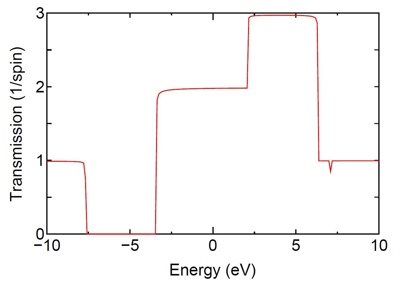
The calculations can be traced by using the input files stored in a directory of 'work/negf_example'. By plotting the sixth column in 'negf-chain.tran0_0' as a function of the fourth column, you can see a transmission curve as shown in Fig. 32.
 |
2016-04-03