Next: Initial Hessian for the Up: Geometry optimization Previous: Steepest decent optimization Contents Index
Although 'Opt' is a robust scheme, the convergence speed can be slow in general. Faster schemes based on quasi Newton methods are available for the geometry optimization. They are the eigenvector following (EF) method [47], the Broyden-Fletcher-Goldfarb-Shanno (BFGS) method [49], the rational function (RF) method [48], and a direct inversion iterative sub-space (DIIS) method [46], implemented in Cartesian coordinate. In the EF and RF methods, the approximate Hessian is updated by the BFGS method. Thus, five geometry optimizers, Opt, EF, BFGS, RF and DIIS, are available in OpenMX Ver. 3.8, which can be specified by 'MD.Type'. The relevant keywords are listed below:
   MD.Type                     EF         # Opt|DIIS|BFGS|RF|EF
   MD.Opt.DIIS.History          3         # default=3
   MD.Opt.StartDIIS             5         # default=5
   MD.Opt.EveryDIIS            200        # default=200
   MD.maxIter                  100        # default=1
   MD.Opt.criterion          1.0e-4       # default=0.0003 (Hartree/Bohr)
   MD.Opt.DIIS.History      3       # default=3
   MD.Opt.StartDIIS         5       # default=5
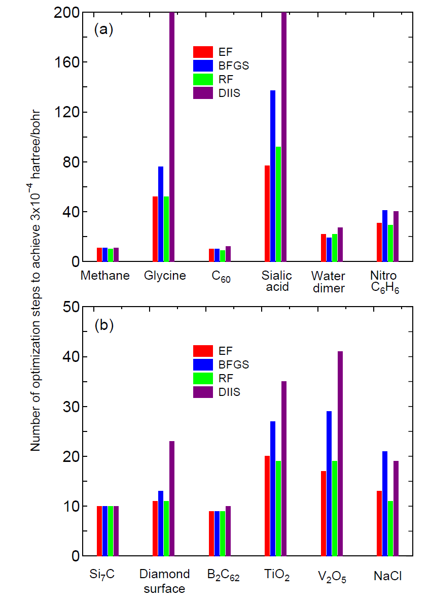
The initial step in the optimization is automatically tuned by monitoring the maximum force in the initial structure. As shown in Fig. 10 which shows the number of geometry steps to achieve the maximum force of below 0.0003 Hartree/Bohr in molecules and bulks, in most cases the RF method seems to be the most robust and efficient scheme, while the EF and BFGS methods also show a similar performance. The input files used for those calculations and the out files can be found in the directory 'work/geoopt_example/'.
It should be also noted that by these quasi Newton methods geometrical structures tend to be converged to a saddle point rather than a stationary minimum point. This is because the structure at which the quasi Newton method started to be employed does not reach at a flexion point. In such a case, the structure should be optimized well by the steepest decent method before moving to the quasi Newton method. The treatment can be easily done by only taking a larger value for 'MD.Opt.StartDIIS', or by restarting the calculation using a file 'System.Name.dat#', where 'System.Name' is 'System.Name' specified in your input file.
In general, a faster convergence can be obtained by employing a large 'scf.energycutoff' leading to a smooth energy curve. This situation is apparent especially for weakly interacting systems such as molecular solids. We recommend for users to employ a large 'scf.energycutoff', e.g., 300-400 Ryd for such a system.
 |