Conventional scheme

The density of states (DOS) is calculated by the following two steps:

(1) SCF calculation

Let us illustrate the calculation of DOS using the carbon diamond. In a file 'Cdia.dat' in the directory 'work', the keywords for the DOS calculation are set to

    Dos.fileout                  on      
    Dos.Erange              -25.0  20.0  
    Dos.Kgrid                12 12 12

In the specification of the keyword 'Dos.Erange', the first and second values are the lower and upper bounds of the energy range (eV) for the DOS calculation, respectively, where the origin (0.0) of energy corresponds to the chemical potential. Also, in the specification of the keyword 'Dos.Kgrid', a set of numbers (n1,n2,n3) is the number of grids to discretize the first Brillouin zone in the k-space, which is used in the DOS calculation. Then, we execute OpenMX by:

    % ./openmx Cdia.dat
  

When the execution is completed normally, then you can find files 'cdia.Dos.val' and 'cdia.Dos.vec' in the directory 'work'. The eigenvalues and eigenvectors are stored in the files 'cdia.Dos.val' and 'cdia.Dos.vec' in a text and binary forms, respectively. The DOS calculation is supported even for the O($N$) calculation, while a Gaussian broadening method is employed in this case.

(2) Calculation of the DOS

Let us compile a program package for calculating DOS. Move the directory 'source', and then compile as follows:

    % make DosMain
  

When the compile is completed normally, then you can find an executable file 'DosMain' in the directory 'source'. Please copy the file 'DosMain' to the directory 'work', and then move to the directory 'work'. You can calculate DOS and projected DOS (PDOS) using the program 'DosMain' from two files 'cdia.Dos.val' and 'cdia.Dos.vec' as:

    % ./DosMain cdia.Dos.val cdia.Dos.vec
  

Then, you are interactively asked from the program as follow:

    % ./DosMain cdia.Dos.val cdia.Dos.vec
    Max of Spe_Total_CNO = 8
    1 1 101 102 103 101 102 103
    <cdia.Dos.val>
    <cdia>
    Which method do you use?, Tetrahedron(1), Gaussian Broadeninig(2)
    1
    Do you want Dos(1) or PDos(2)?
    2

    Number of atoms=2
    Which atoms for PDOS : (1,...,2), ex 1 2
    1
    pdos_n=1
    1
    <Spectra_Tetrahedron> start
    Spe_Num_Relation 0 0 1
    Spe_Num_Relation 0 1 1
    Spe_Num_Relation 0 2 101
    Spe_Num_Relation 0 3 102
    Spe_Num_Relation 0 4 103
    Spe_Num_Relation 0 5 101
    Spe_Num_Relation 0 6 102
    Spe_Num_Relation 0 7 103
    make cdia.PDOS.Tetrahedron.atom1.s1
    make cdia.PDOS.Tetrahedron.atom1.p1
    make cdia.PDOS.Tetrahedron.atom1.p2
    make cdia.PDOS.Tetrahedron.atom1.p3
    make cdia.PDOS.Tetrahedron.atom1

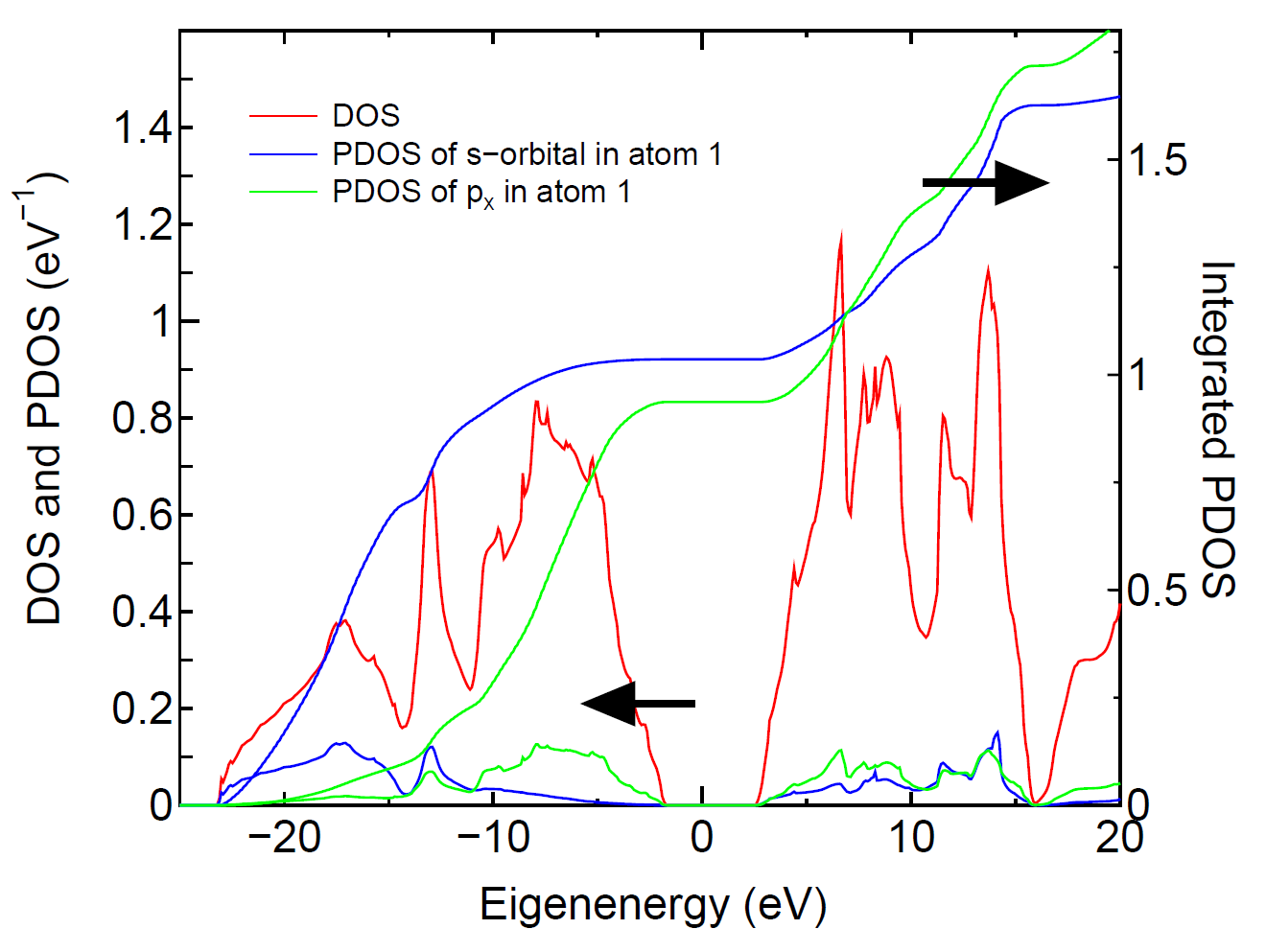
The tetrahedron [51] and Gaussian broadening methods for evaluating DOS are available. Also, you can select DOS or PDOS. When you select the calculation of PDOS, then please select atoms for evaluating PDOS. In this case, each DOS projected on orbitals (s, px (p1), py (p2), pz (p3),..) in selected atoms are output in each file. In these files, the first and second columns are energy in eV and DOS (eV$^{-1}$) or PDOS (eV$^{-1}$), and the third column is the integrated DOS or PDOS. If a spin-polarized calculation using 'LSDA-CA', 'LSDA-PW', or 'GGA-PBE' is employed in the SCF calculation, the second and third columns in these files correspond to DOS or PDOS for up and down spin states, and the fourth and fifth columns are the corresponding integrated values. If you select the Gaussian broadening method, you are requested to set a parameter, value of Gaussian, a (eV), which determines the width of Gaussian defined by $\exp( -(E/a)^2 )$. Figure 15 shows DOS and PDOS of carbon diamond.

Figure 15: DOS and PDOS of the carbon diamond, and the integrated PDOS, where the Fermi level is set to zero. Since charge redistribution occurs among the s-, p-, and d-orbitals, the integrated PDOS of s- and p-orbitals at the Fermi level are not exactly 1. The calculation can be traced by using an input file 'Cdia.dat' in the directory 'work'.