The  invariant of the system can be calculated with a method based on the Berry phase formalism
proposed by Fukui and Hatsugai [81,82].
The functionality is compatible with only the non-collinear calculations.
Also, magnetic systems cannot be treated by the current implementation.
To acknowledge in any publications by using the functionality,
the citation of the reference [84] would be appreciated.
invariant of the system can be calculated with a method based on the Berry phase formalism
proposed by Fukui and Hatsugai [81,82].
The functionality is compatible with only the non-collinear calculations.
Also, magnetic systems cannot be treated by the current implementation.
To acknowledge in any publications by using the functionality,
the citation of the reference [84] would be appreciated.
The invariant is a topological invariant number being 0 or 1, which is defined
on time reversal symmetric non-magnetic systems.
 and
and  correspond to topological and trivial insulators, respectively.
The invariant is defined as
correspond to topological and trivial insulators, respectively.
The invariant is defined as
where
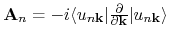 is called Berry connection, and
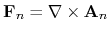 is called Berry curvature.
The integration range
is called Berry curvature.
The integration range
![$B=[-\frac{{\bf G}_{1}}{2},\frac{{\bf G}_{1}}{2}]\otimes[0,\frac{{\bf G}_{2}}{2}]$](img468.png) is enough to consider only the half of Brillouin zone.
This is because the system has the time-reversal symmetry, and thereby the topological invariant
is defined on the half of Brillouin zone.
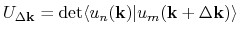
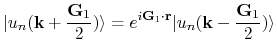
For performing the integration, we use the overlap matrix
is enough to consider only the half of Brillouin zone.
This is because the system has the time-reversal symmetry, and thereby the topological invariant
is defined on the half of Brillouin zone.
For performing the integration, we use the overlap matrix  , proposed by Fukui, Hatsugai, and Suzuki
[81,82],
defined by
, proposed by Fukui, Hatsugai, and Suzuki
[81,82],
defined by
 ,
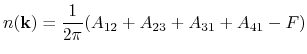
and calculate the Berry connection and Berry curvature on every 'plaquette',
which means meshed area in the Brillouin zone, as
,
and calculate the Berry connection and Berry curvature on every 'plaquette',
which means meshed area in the Brillouin zone, as
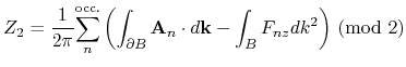
Then, the integer-valued field  on every plaquette can be calculated by the following formula;
By summing up all the  on the half Brillouin zone, and considering the modulo 2 of the summed value,
we can obtain the invariant. It should be noted that the invariant is gauge independent,
but the value of each is gauge dependent, which may vary depending on computational environment,
compiler optimization level, and a tiny difference in the electronic structure.
The details of computing
on the half Brillouin zone, and considering the modulo 2 of the summed value,
we can obtain the invariant. It should be noted that the invariant is gauge independent,
but the value of each is gauge dependent, which may vary depending on computational environment,
compiler optimization level, and a tiny difference in the electronic structure.
The details of computing  and
and  is explained in Section of "Chern number and Berry curvature".
Please refer it.
Since the calculation of the invariant is carried out by the contour integral
on the half of Brillouin zone, it depends on arbitrariness of wave function's gauges.
Therefore, we have to fix the gauges on the boundary of half Brillouin zone.
As shown in Fig. 75, we consider the following three kinds of gauge fix on the boundary:
is explained in Section of "Chern number and Berry curvature".
Please refer it.
Since the calculation of the invariant is carried out by the contour integral
on the half of Brillouin zone, it depends on arbitrariness of wave function's gauges.
Therefore, we have to fix the gauges on the boundary of half Brillouin zone.
As shown in Fig. 75, we consider the following three kinds of gauge fix on the boundary:
Translational symmetry (red parts)
Time-reversal symmetry (blue parts)
Kramars degenerates (yellow points)
In this calcuation, the eigenvalue problems are solved on the half of integration interval,
in other words, the quarter of Brillouin zone as shown in Fig. 75.
Figure 75:
Gauge fixing on the half Brillouin zone. We fix the wavefunction's gauges
as red parts satisfying the translational symmetry,
blue parts satisfying the time-reversal symmetry,
and yellow points satisfying the Kramars degeneracies.
|
|
When we perform the integrals on the other area,
we generate wave functions by fixing wavefunction's gauges
on the symmetrically corresponding plaquette, and perform the integral.
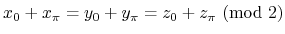
In case of the three dimensional system, the Brillouin zone has six time-reversal invariant planes,
 ,
,
 (
( ).
Thus, six invariants (
).
Thus, six invariants (
 )
can be defined as shown in Fig. 76.
Note that these invariants satisfy the following equation:
)
can be defined as shown in Fig. 76.
Note that these invariants satisfy the following equation:
Therefore, only four invariants become independent parameters.
Based on the fact, the invariant in 3D system is defined as
Especially, the system of  is called strong topological insulator
because the state appears on all the direction in the Brillouin zone.
is called strong topological insulator
because the state appears on all the direction in the Brillouin zone.
Figure 76:
The six invariants defined on 3D reciprocal lattice space.
These invariants satisfy
 ,
and only four invariants become independent parameters.
,
and only four invariants become independent parameters.
|
|
![\includegraphics[width=8.0cm]{Z2-Fig1.eps}](img481.png)
![\includegraphics[width=12.0cm]{Z2-Fig2.eps}](img489.png)