what's new up

What's New

12/Oct./2023

The 4th OpenMX developer's meeting in ISSP

The 4th OpenMX developer's meeting will be held in Institute for Solid State Physics (ISSP), the University of Tokyo, for Nov. 9th and 10th, 2023. Recent development and implementation of new functionalities will be discussed including some advanced applications using OpenMX. The meeting will provide a good opportunity for active developers to exchange their ideas, and promote further development of OpenMX. We also encourage researchers, who are interested in contributing to development of OpenMX, to attend the informal meeting. We are looking forward to having stimulating discussion in ISSP.

If you wish to attend the meeting, please send an email to t-ozaki@issp.u-tokyo.ac.jp, including your name and affiliation.

The information of the meeting will be updated on the website.

17/Oct./2021

The patch (Ver.3.9.9) to OpenMX Ver. 3.9 has been released.

A patch 3.9.9 to OpenMX Ver. 3.9 has been released at patch3.9.9.tar.gz. Related to Cluster_DFT_Col.c: The calculation of the partial charge was not properly performed when only the Gamma point is employed. The bug has been fixed by applying the patch. All the purpose of the patch and how to apply it can be found at README.

Thank you very much for your cooperation in advance.

28/Sep./2021

The patch (Ver.3.9.8) to OpenMX Ver. 3.9 has been released.

A patch 3.9.8 to OpenMX Ver. 3.9 has been released at patch3.9.8.tar.gz. A bug related to DFT-D2 and DFT-D3 has been fixed. All the purpose of the patch and how to apply it can be found at README.

Thank you very much for your cooperation in advance.

15/Sep./2021

The patch (Ver.3.9.7) to OpenMX Ver. 3.9 has been released.

A patch 3.9.7 to OpenMX Ver. 3.9 has been released at patch3.9.7.tar.gz. An instability issue of DFT-D2 and DFT-D3 has been fixed and the variable cell optimization including DFT-D2 and DFT-D3 has been supported. Also, the compilation issue of MulPOnly has been fixed. All the purpose of the patch and how to apply it can be found at README.

Thank you very much for your cooperation in advance.

21/Aug./2021

The patch (Ver.3.9.6) to OpenMX Ver. 3.9 has been released.

A patch 3.9.6 to OpenMX Ver. 3.9 has been released at patch3.9.6.tar.gz, where an instability issue of force calculation using the hybrid parallelization using MPI and OpenMP has been fixed. The purpose of the patch and how to apply it can be found at README.

Thank you very much for your cooperation in advance.

14/Aug./2021

The patch (Ver.3.9.5) to OpenMX Ver. 3.9 has been released.

A patch 3.9.5 to OpenMX Ver. 3.9 has been released at patch3.9.5.tar.gz, since the directory structure of the patch 3.9.4, released on Aug. 14th, 2021, may cause a trouble in the re-installation. The purpose of the patch and how to apply it can be found at README.

Thank you very much for your cooperation in advance.

14/Aug./2021

The patch (Ver.3.9.4) to OpenMX Ver. 3.9 has been released.

A patch 3.9.4 to OpenMX Ver. 3.9 has been released at patch3.9.4.tar.gz. The purpose of the patch and how to apply it can be found at README.
Since the patch 3.9.3, released on Aug. 13th, 2021, does not include the following files: MulPOnly.c, Occupation_Number_LDA_U.c, TRAN_Add_Density_Lead.c, and neb_run.c, which have been patched by the patch 3.9.2, they are also included in the patch 3.9.4.

Thank you very much for your cooperation in advance.

13/Aug./2021

The patch (Ver.3.9.3) to OpenMX Ver. 3.9 has been released.

A patch 3.9.3 to OpenMX Ver. 3.9 has been released at patch3.9.3.tar.gz.
The purpose of the patch and how to apply it can be found at README.

Thank you very much for your cooperation in advance.

11/Feb./2020

The patch (Ver.3.9.2) to OpenMX Ver. 3.9 has been released.

A patch 3.9.2 to OpenMX Ver. 3.9 has been released at patch3.9.2.tar.gz.
The purpose of the patch and how to apply it can be found at README.

Thank you very much for your cooperation in advance.

02/Jan./2020

The patch (Ver.3.9.1) to OpenMX Ver. 3.9 has been released.

A patch 3.9.1 to OpenMX Ver. 3.9 has been released at patch3.9.1.tar.gz.
The purpose of the patch and how to apply it can be found at README.

Thank you very much for your cooperation in advance.

03/Dec./2019

OpenMX Ver 3.9 (with user's manual) has been released.

The main features (PDF) of the development are as follows:
    (1) Database (2019) of VPS and PAO (supported by T. Ozaki)

      The database of fully relativistic pseudopotentials (VPS) and optimized pseudo-atomic orbitals (PAO) files has been updated as Database (2019), and distributed with OpenMX Ver. 3.9. Though the most of data are the same as in Ver. 2013, the VPS and PAO files for Fe, Os, Tc, La, Ce, Pr, and Pm are updated. The mean delta gauge of 71 elements in the database Ver. 2019 is 1.774 meV/atom with the standard deviation of 1.702 meV/atom. Related information can be found in the Database (2019).
    (2) Database (2019) of VPS and PAO for core excitations (supported by T. Ozaki)

      The database of fully relativistic pseudopotentials (VPS) and pseudo-atomic orbitals (PAO) which can be used for calculations of core level excitations has been released as Database (2019) for core excitations. The data for B, C, N, O, Si, S, Ge, Pt elements are available. When you calculate absolute binding energies of core levels in bulk and gaseous systems, which can be measured in X-ray photoemission spectroscopy (XPS), the VPS and PAO files have to be used. Related information can be found in the Database (2019) for core excitations and XPS core level energies.
    (3) Requirement of ScaLAPACK and BLACS (supported by T. Ozaki)

      The installation of OpenMX Ver. 3.9 requires linking of ScaLAPACK, BLACS, and a MPI library, while OpenMX Ver. 3.8 can be compiled with LAPACK and BLAS. Please note that the compilation of OpenMX Ver. 3.9 with LAPACK and BLAS is not supported anymore. Related information can be found in the Installation.
    (4) Absolute binding energies of core levels: XPS core level energies (supported by T. Ozaki)

      A general method has been supported to calculate absolute binding energies of core levels in metals and insulators, based on a penalty functional and an exact Coulomb cutoff method in the framework of density functional theory. With the method the spurious interaction of core holes between supercells is avoided by the exact Coulomb cutoff method, while the variational penalty functional enables us to treat multiple splittings due to chemical shift, spin-orbit coupling, and exchange interaction on equal footing. It has been demonstrated that the absolute binding energies of core levels for both metals and insulators are calculated by the proposed method in a mean absolute (relative) error of 0.4 eV (0.16%) for eight cases compared to experimental values measured with x-ray photoemission spectroscopy (XPS) within a generalized gradient approximation to the exchange-correlation functional. The calculations require fully relativistic pseudopotentials (VPS) and optimized pseudo-atomic orbitals (PAO) files including the targeted core level. Related information can be found in the XPS core level energies.
    (5) Divide-conquer method with localized natural orbitals (DC-LNO) method (supported by T. Ozaki)

      An efficient O(N) divide-conquer (DC) method based on localized single-particle natural orbitals (LNOs) has been released for large-scale density functional theory (DFT) calculations of gapped and metallic systems. The LNOs are noniteratively calculated by a low-rank approximation via a local eigendecomposition of a projection operator for the occupied space. Introducing LNOs to represent the long-range region of a truncated cluster reduces the computational cost of the DC method while keeping computational accuracy. A series of benchmark calculations and high parallel efficiency in a multilevel parallelization clearly demonstrate that the O(N) method enables us to perform large-scale simulations for a wide variety of materials including metals with sufficient accuracy in accordance with development of massively parallel computers. Related information can be found in the O(N) DC-LNO method.
    (6) Ionization potential and electron affinity of gaseous systems (supported by T. Ozaki)

      The ionization potential and electron affinity of gaseous systems can be calculated by a delta SCF method with an exact Coulomb cutoff method. With the exact Coulomb cutoff method, a calculation of a charged isolated system is possible even in the periodic boundary condition. What you need is to perform two calculations for the ground and ionized states of an isolated system, and to calculate the difference of the total energies between them. Related information can be found in the Ionization potential and electron affinity of gaseous systems.
    (7) Optical conductivity and dielectric function (supported by Y-.T. Lee and T. Ozaki)

      In OpenMX Ver. 3.9, the conductivity and dielectric function can be calculated based on the Kubo-Greenwood formula. Starting from the Born approximation, the complex tensor of conductivity and dielectric function, which are frequency dependent, are calculated within a linear response to a perturbing frequency dependent electric field. Other physical quantities such as absorption, extinction, transmission, reflection, and refractive index are also calculated, which are all derived from the conductivity. The functionality is compatible with only collinear calculations. The extension of the functionality to the non-collinear case will be supported in the future release. Since the multi-level parallelization has been implemented, it is possible to perform large-scale calculations of systems including more than 1000 atoms on massively parallel computers. Related information can be found in the Optical conductivity and dielectric function.
    (8) Analysis of spin texture (supported by H. Kotaka, N. Yamaguchi, and F. Ishii)

      Spin splitting in the band structure as can be seen in the Rashba effect may occur when the spin-orbit coupling is taken into account. The spin splitting can be resolved in each state and the a wave vector k, and the state- and k-resolved spin splitting, which is a spin structure on the band dispersion relation in the reciprocal space, is called spin texture. Using a post-processing code 'kSpin' one can calculate the spin texture in the case of a non-collinear calculation with spin-orbit coupling. The state- and k-resolved spin density matrix, which is referred to as the k-space spin density matrix hereafter, is calculated from the two component spinor, and takes a form of a 2x2 matrix. The spin texture is actually calculated using the 2x2 matrix. In addition to the spin texture, 'kSpin' provides us the k-space spin density matrix so that physical origins of phenomena caused by spin-orbit interaction such as the Rashba effect can be analyzed. 'kSpin' also supports the analysis of spin texture resolved for not only each state and the a wave vector k, but also atom and pseudo-atomic orbital, which may help us to understand which atom and orbital play a central role of the spin splitting. Note that 'kSpin' is applicable to not only the Rashba effect but also topological insulators and systems with non-Rashba type spin splitting. Related information can be found in the Analysis of spin texture in the k-space .
    (9) Chern number, Berry curvature, and Z2 invariant (supported by H. Sawahata and F. Ishii)

      In OpenMX Ver. 3.9, a post-processing code 'calB' is supported to calculate the Chern number and Berry curvature of bands using overlap matrix elements between Kohn-Sham orbitals at neighboring k-points by the Fukui-Hatsugai-Suzuki method. The Chern number is a topological invariant being an integer number, which characterizes the topology of bands for magnetic materials. We also release another post-processing code 'Z2FH' to calculate the Z2 topological invariant using the Berry phase by the Fukui-Hatsugai method. Related information can be found in the Computing Chern number and Berry curvature by Fukui-Hatsugai-Suzuki method. Computing Z2 invariant by Fukui-Hatsugai method.
    (10) Generalized Bloch theory for spin spiral (supported by T.B. Prayitno and F. Ishii)

      Spin spiral calculations are supported for the non-collinear DFT without spin orbit coupling (SOC), which is based on the generalized Bloch theorem. It should also be stressed that the inclusion of SOC is not compatible with the functionality, since the SOC violates the spiral symmetry imposed by the generalized Bloch theorem. With the functionality one can calculate spin spiral magnetic structures which may have an incommensurate periodicity with repect to the lattice periodicity. Related information can be found in the Spin spiral calculations .
    (11) Improvement of polB (supported by N. Yamaguchi)

      A post-processing code 'polB' to calculate electric polarization based on the Berry phase formalism has been improved with respect to efficienty and stability. Related information can be found in the Macroscopic polarization by Berry's phase .
    (12) Second variational method: Magnetic Anisotropy Energy (MAE) (supported by P.-H. Chang and T. Ozaki)

      A second variational method is supported to calculate band structures modified with spin-orbit coupling (SOI) and magnetic anisotropy energy (MAE). This is based on the Harris functional which is a perturbation theory for evaluating the total energy. Using the SCF charge density calculated by the collinear DFT one can calculate the band structure and the band energy by the one-shot diagonalization for the Hamiltonian with SOI. The second variational method is an efficient approach for the evaluation of MAE by considering the accuracy and efficiency. The second variational scheme might be useful for not only the evaluation of MAE, but also calculations of band structure of large-scale systems, which may hamper direct SCF calculations by the non-collinear DFT method, to investigate how the SOI modifies the band structure. Related information can be found in the Second variational method: Magnetic Anisotropy Energy (MAE) .
    (13) Efficient calculations of exchange coupling parameters (supported by A. Terasawa, T. Ozaki, and Y. Gohda)

      A post-processing code 'jx' to calculate exchange coupling parameters Jij has been largely improved so that the individual Jij in bulks can be calculated efficiently using a contour integration method. The code will be utilized for analysis of the individual effective exchange coupling parameters not only in isolated systems but also bulks on an equal footing. The details of the improvement has been published in a paper . Related information can be found in the Exchange coupling parameters .
    (14) Optimization of enthalpy (supported by T. Ozaki)

      It is possible to perform the variable cell optimization under an applied pressure. This is done by minimizing the enthalpy H=E+pV, where E is the total energy, p the applied pressure, V the volume of the unit cell. Applying the anisotropic pressure is also possible by choosing designated axes. Related information can be found in the Optimization of enthalpy .
    (15) Generalized DFT+U methods (supported by S. Ryee and M.J. Han)

      In addition to the simplified rotationally invariant form supported by OpenMX Ver. 3.8, general forms of the DFT+U methods are supported with respect to the occupation number operator, the functional form, and the choice of the double counting term for both the collinear and noncollinear calculations. In the general DFT+U schemes, not only U but also J (Hund's coupling J) are explicitly introduced as input parameters. Also, a fully localized limit (FLL) and around mean-field (AMF) for the treatment of the double-counting term are introduced with a combination with the density functional scheme within charge (spin-unpolarized) density and spin density LDA/GGA, which can be specified as 'sFLL', 'sAMF', 'cFLL', and 'cAMF'. Related information can be found in the DFT+U methods .
    (16) RMM-DIIS mixing for the Kohn-Sham potentials (supported by T. Ozaki)

      A residual minimization method in the direct inversion iterative subspace (RMM-DIISV) for the Kohn-Sham potentials is supported for the SCF calculations. Our benchmark calculations imply that the performance of RMM-DIISV seems to be comparable to RMM-DIISK, while the RMM-DIISV outperforms the other mixing methods in some cases. Related information can be found in the SCF convergence .
    (17) Variable cell optimization with constraints (supported by T. Ozaki)

      Variable cell optimization methods with new constraints are supported as 'OptC6', 'OptC7', 'RFC6', and 'RFC7'. 'OptC6' is a method that cell vectors and internal coordinates are simultaneously optimized with a constraint that a cell vector a3 is fixed, while 'OptC7' introduces a constraint that two cell vectors a2 and a3 are fixed. In 'OptC6' and 'OptC7' the optimization is performed with a steepest decent method with a variable prefactor. 'RFC6' and 'RFC7' behave just like 'OptC6' and 'OptC7', respectively. However, the optimization is performed with the rational function (RF) method. Related information can be found in the Variable cell optimization .
    (18) Calculations of work functions (supported by N. Yamaguchi and T. Ozaki)

      We illustrate how to calculate work functions using cube files of either System.Name.v0.cube or System.Name.v1.cube. The calculations of work function for surfaces of five metals are demonstrated including an issue that how we should introduce the empty layers to take account of the tail of wave function towards the vacuum region. A small utility program 'gcube2oned.c', which transforms the data of 3D cube data to an 1D data along a chosen direction by averaging over the remaining plane, is also released for user's convenience. Related information can be found in the Calculations of work functions .
    (19) Calling OpenMX as library or computational engine (supported by T. Ozaki)

      OpenMX can be utilized as library or computational engine from your program using MPI_Comm_spawn. You may mpirun your program and may want to call OpenMX with different input files from the program in different MPI groups at the same time. In such cases the functionality may be useful. Since an example code how to utilize the functionality is provided, you may easily start to use the functionality. Related information can be found in the Calling OpenMX as library or computational engine.
    (20) Interface with BoltzTraP (supported by M. Miyata)

      OpenMX is interfaced with BoltzTraP which calculates electron transport coefficients based on the Boltzmann theory from the wave number dependence of the energy eigenvalues in the Kohn-Sham equation. The interface with BoltzTraP enables us to calculate physical properties such as the Seebeck coefficient, electrical conductivity, electronic thermal conductivity, and the Hall coefficient. The functionality is compatible with not only the collinear calculations, but also the non-collinear calculations. Related information can be found in the Interface with BoltzTraP.
    (21) Change of the data format for the scfout file (supported by N. Yamaguchi and T. Ozaki)

      Via the scfout file one can access the computational data such as the matrix elements for the Hamiltonian, overlap, density matrix, position operator, and momentum operator, which are all obtained from the SCF calculation. The functionality allows us to develop a post processing code which utilizes these data. In the release of OpenMX Ver. 3.9, the data format for the relevant codes 'SCF2File.c', 'read_scfout.c', 'read_scfout.h', and 'analysis_example' have been changed so that the full information of density matrix, and the matrices for the position operator and momentum operator can be included in the scfout file. So, note that the scfout files generated by the older versions of OpenMX cannot be analyzed by Ver. 3.9. Related information can be found in the Interface for developers.
    (22) Choice of the axis to be treated by ESM method (supported by M. Otani)

      In OpenMX Ver. 3.8, the treatment by the ESM method is applied to the x-axis, and the other choice is not allowed. OpenMX Ver. 3.9 supports arbitrary choice (x, y, or z) of the axis to be treated by ESM method by the keyword 'ESM.direction' as
          ESM.direction            x         # x|y|z, default=x          
         
      The default direction is the x-axis. Related information can be found in the Effective screening medium method.
    (23) A set of choices for the PAO basis functions (supported by T. Ozaki)

      For user's convenience, a set of proper choices for the basis functions is provided in Tables of the manual. For each pseudopotential, three choices: Quick, Standard, and Precise are given in the Tables. Quick allows us a quick calculation, but with a reasonably accuracy. Standard can be a proper choice for the most of users, which balances the accuracy and efficiency. Precise almost reaches to convergent results in most of cases. The tables give a guideline in choosing the basis functions, while of course, basis functions can be properly selected depending on your purpose. Related information can be found in the choices for PAOs.
    (24) ELPA1 and ELPA2 (supported by T.V.T. Duy and T. Ozaki)

      For the cluster and band diagonalization methods, either ELPA1 or ELPA2 can be chosen by the following keyword:
          scf.eigen.lib      elpa1    # elpa1|elpa2, default=elpa1
       
      The default choice is ELPA1. Our benchmark calculations suggest that ELPA1 and ELPA2 are comparable to each other with respect to the computational speed. Related information can be found in the ELPA| ELPA.
    (25) Memory reduction for the cluster and band calculations (supported by T. Ozaki)

      The memory requirement for the cluster and band calculations including the calculation of density of states (DOS) has been improved. Compared to OpenMX Ver. 3.8, the memory requirement for the calculations is reduced especially in large-scale calculations. There is no additional keyword for the improvement.
    (26) Interface with FermiSurfer (supported by M. Kawamura)

      To visualize Fermi surfaces, OpenMX generates files which can be readable by FermiSurfer (http://fermisurfer.osdn.jp/). Related information can be found in the Fermi surface.
    (27) Graphical User Interface (GUI) and/or job scheduling environment

      A couple of GUIs and job scheduling environments for OpenMX calculations are available as follows:

    (28) Bugs fixed

      Minor bugs in OpenMX Ver. 3.8 were fixed.
    (29) Manual revised

      The manual of OpenMX was revised.

12/June/2018

The patch (Ver.3.8.5) to OpenMX Ver. 3.8 was released.

A patch 3.8.5 to OpenMX Ver. 3.8 was released at patch3.8.5.tar.gz.
The purpose of the patch and how to apply it can be found at README.

Thank you very much for your cooperation in advance.

05/March/2018

The patch (Ver.3.8.4) to OpenMX Ver. 3.8 was released.

A patch 3.8.4 to OpenMX Ver. 3.8 was released at patch3.8.4.tar.gz.
The purpose of the patch and how to apply it can be found at README.

Thank you very much for your cooperation in advance.

08/March/2017

The patch (Ver.3.8.3) to OpenMX Ver. 3.8 was released.

A patch 3.8.3 to OpenMX Ver. 3.8 was released at patch3.8.3.tar.gz.
The purpose of the patch and how to apply it can be found at README.

Thank you very much for your cooperation in advance.

02/March/2017

The patch (Ver.3.8.2) to OpenMX Ver. 3.8 was released.

A patch 3.8.2 to OpenMX Ver. 3.8 was released at patch3.8.2.tar.gz.
The purpose of the patch and how to apply it can be found at README.

Thank you very much for your cooperation in advance.

21/Oct./2016

The patch (Ver.3.8.1) to OpenMX Ver. 3.8 was released.

A patch 3.8.1 to OpenMX Ver. 3.8 was released at patch3.8.1.tar.gz.
The purpose of the patch and how to apply it can be found at README.

Thank you very much for your cooperation in advance.

19/Aug./2016

OpenMX Viewer was released.

A web-based graphical user interface (GUI), OpenMX Viewer Ver. 1.0, was released under the practice of the GNU General Public License v3 (GPL). The web-based GUI enables us to quickly visualize crystal and molecular structures in input and output files of OpenMX by simply drag and drop, and analyze structural parameters such as bond length and bond angle in a convenient way. Several basic functionalities such as analysis of Mulliken charges, molecular dynamics, and geometry optimization are also available. In the Ver. 1.0 supported formats of files are the input file 'dat' and output files 'xyz', and 'md' file generated by OpenMX Ver. 3.8. To enhance the usability of OpenMX Viewer, the use of Google Chrome is highly recommended due to its performance. The update of OpenMX Viewer will be made occasionally without official announcement except for a case of major revision. We hope that OpenMX Viewer will be helpful for your researches.

03/April/2016

OpenMX Ver 3.8 (with user's manual) was released.

The main features of the development are as follows:
    (1) Unfolding method for band structures (supported by C.-C. Lee and T. Ozaki)

      In OpenMX Ver. 3.8, an unfolding method for band structures is released, of which implementation details is found in J. Phys.: Condens. Matter 25, 345501 (2013). When the band structure of a system with imperfection such as surfaces, impurities, vacancies, and structural distortion calculated by the supercell approach is compared to spectrum measured by Angle-Resolved Photoemission Spectroscopy (ARPES), the experimentally measured periodicity of the system is generally different from that of the supercell we introduced for the calculation. OpenMX provides a method for unfolding the band structure of the supercell into the Brillouin zone of a reference unit cell that a user specifies in the input file. The functionality is supported for not only collinear, but also non-collinear DFT calculations. Related information can be found in the manual.
    (2) DFT-D3 method for vdW interaction (supported by M. Ellner and R. Perez)

      The DFT-D3 method by Grimme et al. (J. Chem. Phys. 132, 154104 (2010)) is supported to include a vdW interaction as well as the DFT-D2 method (J. Comput. Chem. 27, 1787 (2006)). The usage of the functionality can be found in the manual.
    (3) Analysis of real-space charge/spin current density (supported by M. Kawamura, K. Yoshimi, and T. Ozaki)

      OpenMX Ver. 3.8 supports a tool to analyze how charge and spin current flow in real space by calculating the real-space charge and spin current density. The usage of the functionality can be found in the manual. Also the technical notes on the implementation can be found in here.
    (4) Analysis of eigenchannels for electric transport (supported by M. Kawamura, K. Yoshimi, and T. Ozaki)

      OpenMX Ver. 3.8 provides an analysis tool to investigate how charge and spin current flow through eigenchannels of transmission. The usage of the functionality can be found in the manual. Also the technical notes on the implementation can be found in here.
    (5) Variable cell optimization (supported by Y. Shiihara and T. Ozaki)

      Variable cell optimizations with/without constraints are available in OpenMX Ver. 3.8. Not only full optimization for cell vectors and internal coordinates, but also constraint optimization for the cell shape are supported. The usage of the functionality can be found in the manual.
    (6) Initial approximate Hessian (supported by T. Ozaki)

      OpenMX Ver. 3.8 supports an initial approximate Hessian, proposed by Schlegel (Theoret. Chim. Acta (Berl.) 66, 333 (1984); J. Mol. Struc. (Theochem) 398-399, 55 (1997)), for the RF and EF optimizers in the geometry and variable cell optimizations. The initial approximate Hessian may substantially accelerate the convergence compared to the simplest initial approximate Hessian of the identity. The usage of the functionality can be found in the manual.
    (7) Orbitally decomposed total energy (supported by T. Ozaki)

      OpenMX Ver. 3.8 provides a useful tool which decomposes the total energy into each contribution associated with each basis function, where the decomposition is performed based on projection onto basis functions. The usage of the functionality can be found in the manual.
    (8) ScaLAPACK version of OpenMX (supported by T.V.T. Duy)

      It is possible to enhance the performance of OpenMX using ScaLAPACK, PBLAS, and BLACS. The performance improvement will be obtained in terms of not only computational speed, but also memory usage when 'Cluster' and 'Band' for the keyword 'scf.EigenvalueSolver' is employed for large-scale systems including more than 500 atoms. The usage of the functionality can be found in the here and here
    (9) Natural population analysis (supported by T. Ohwaki)

      In the natural bond orbital (NBO) method developed by Weinhold et al. (Chem. Rev. 88, 899 (1988); WIREs Comput. Mol. Sci. 2, 1 (2012)), atomic population (or atomic charge) is calculated based on atomically localized orbitals, natural atomic orbitals (NAO), which is referred to as natural population (NP). OpenMX supports the NP analysis. Especially, for large-sized calculation models, one can efficiently calculate and analyze NPs by selecting target atoms, which is an original scheme based on a truncated cluster method (J. Chem. Phys. 140, 244105 (2014)). The usage of the functionality can be found in the manual
    (10) Open core pseudopotentials (supported by T. Ozaki)

      The 4f-states in lanthanide elements are spin-polarized in many cases, and the majority states are located at below a few eV taken from the Fermi level. However, LDAs and GGAs cannot describe the feature of band structures for those materials. Although one way is to perform the plus U method by introducing on-site Coulomb repulsion for the 4f-states in such a case, OpenMX Ver. 3.8 provides a simpler way that the spin-polarizaion of 4f-states is taken into account via a pseudopotential, so-called open core pseudopotential, while a few open core pseudopotentials are available in the database Ver. 2013. The usage of the functionality can be found in the manual.
    (11) Interface with Wannier90 (supported by Y.P. Mizuta and F. Ishii)

      OpenMX Ver. 3.8 interfaces with Wannier90 (http://www.wannier.org/) which constructs maximally localized Wannier functions, and calculates physical properties such as Wannier projected DOS and bandstructure, Fermi surface, Berry phase related properties (anomalous Hall conductivity, optical conductivity, and orbital magnetization), and thermoelectric properties. The usage of the functionality can be found in the manual.
    (12) Constraint DFT for non-collinear spin orientation (supported by T. Ozaki)

      OpenMX Ver. 3.8 supports a constraint scheme (scf.Constraint.NC.Spin=on2) in the non-collinear calculation that the spin direction and the magnitude of the spin moment are constrained at the initial setting by the keyword 'Atoms.SpeciesAndCoordinates'. The usage of the functionality can be found in the manual.
    (13) Voronoi volume (supported by T. Ozaki)

      The Voronoi volume which is a volume of the Voronoi polyhedron is provided in OpenMX Ver. 3.8 as a supplemental information during the Voronoi charge analysis. The usage of the functionality can be found in the manual.
    (14) DIISH mixing for Hamiltonian (supported by T. Ozaki)

      RMM-DIIS for Kohn-Sham Hamiltonian (DIISH) is supported in OpenMX Ver. 3.8, which may be useful to accelerate the SCF convergence for the LDA+U calculations. The usage of the functionality can be found in the manual.
    (15) Controling of spin-orbit coupling strength (supported by T. Ozaki)

      In OpenMX Ver. 3.8, it is possible to contol the spin-orbit coupling strength using a conventional pseudopotential stored in the database Ver. 2013 without generating a special pseudopotential with a larger or smaller spin-orbit coupling. The usage of the functionality can be found in the manual.
    (16) 'make all' (supported by T. Ozaki)

      All the executable files including post-processing codes can be compiled. The usage of the functionality can be found in the manual.
    (17) md2axsf (supported by T. Ozaki)

      In molecular dynamics simulations or geometry optimization, 'System.Name.md' is generated to save a series of structural change. Although 'System.Name.md' being the xyz format can be read in xmakemol and XCrySDen, the copied cell in periodic systems cannot be displayed. For such a purpose, a small post processing code is available to convert the format from 'xyz' to 'axsf'. The usage of the functionality can be found in the manual.
    (18) 'level.of.stdout 0' (supported by T. Ozaki)

      For the standard output the minimum information is output by specifying 'level.of.stdout 0', which will be useful for long time molecular dynamics simulations.
    (19) Bugs fixed

      Minor bugs in OpenMX Ver. 3.7 were fixed.
    (20) Manual revised

      The manual of OpenMX was revised.

21/Feb./2015

The patch (Ver.3.7.10) to OpenMX Ver. 3.7 was released.

A patch 3.7.10 to OpenMX Ver. 3.7 was released at patch3.7.10.tar.gz, since it turns out that a file 'Band_DFT_Col.c' in the patch (Ver.3.7.9) is corrupted. The purpose of the patch and how to apply it can be found at README.

Thank you very much for your cooperation in advance.

20/Feb./2015

The patch (Ver.3.7.9) to OpenMX Ver. 3.7 was released.

A patch 3.7.9 to OpenMX Ver. 3.7 was released at patch3.7.9.tar.gz.
The purpose of the patch and how to apply it can be found at README.

Thank you very much for your cooperation in advance.

17/Feb./2014

The patch (Ver.3.7.8) to OpenMX Ver. 3.7 was released.

A patch 3.7.8 to OpenMX Ver. 3.7 was released at patch3.7.8.tar.gz.
The purpose of the patch and how to apply it can be found at README.

Thank you very much for your cooperation in advance.

31/Jan./2014

The patch (Ver.3.7.7) to OpenMX Ver. 3.7 was released.

A patch 3.7.7 to OpenMX Ver. 3.7 was released at patch3.7.7.tar.gz.
The purpose of the patch and how to apply it can be found at README.

Thank you very much for your cooperation in advance.

04/Sep./2013

OpenFFT (Ver.1.0) was released.

OpenFFT is an open source parallel library for computing three-dimensional Fast Fourier Transforms (3-D FFTs) of arbitrary input size and complex data. It originates from OpenMX (Open source package for Material eXplorer). OpenFFT adopts a decomposition method that is capable of reusing data when transposing from one dimension to another for reducing the total volume of communication. It is written in C and MPI, with support for Fortran through the Fortran interface, and employs FFTW for computing 1-D FFTs. OpenFFT is freely available under GNU-GPL. For more information, please visit the website.

01/Sep./2013

The patch (Ver.3.7.6) to OpenMX Ver. 3.7 was released.

A patch 3.7.6 to OpenMX Ver. 3.7 was released at patch3.7.6.tar.gz.
The purpose of the patch and how to apply it can be found at README.

Thank you very much for your cooperation in advance.

29/Aug./2013

The patch (Ver.3.7.5) to OpenMX Ver. 3.7 was released.

A patch 3.7.5 to OpenMX Ver. 3.7 was released at patch3.7.5.tar.gz.
The purpose of the patch and how to apply it can be found at README.

Thank you very much for your cooperation in advance.

03/July/2013

The patch (Ver.3.7.4) to OpenMX Ver. 3.7 was released.

A patch 3.7.4 to OpenMX Ver. 3.7 was released at patch3.7.4.tar.gz.
The purpose of the patch and how to apply it can be found at README.

Thank you very much for your cooperation in advance.

03/June/2013

The patch (Ver.3.7.3) to OpenMX Ver. 3.7 was released.

A patch 3.7.3 to OpenMX Ver. 3.7 was released at patch3.7.3.tar.gz.
The purpose of the patch and how to apply it can be found at README.

Thank you very much for your cooperation in advance.

29/May/2013

The patch (Ver.3.7.2) to OpenMX Ver. 3.7 was released.

A patch 3.7.2 to OpenMX Ver. 3.7 was released at patch3.7.2.tar.gz.
The purpose of the patch and how to apply it can be found at README.

Thank you very much for your cooperation in advance.

27/May/2013

The patch (Ver.3.7.1) to OpenMX Ver. 3.7 was released.

A patch 3.7.1 to OpenMX Ver. 3.7 was released at patch3.7.1.tar.gz. When disabling the OpenMP parallelism by -Dnoomp, the compilation will not be completed. Applying the patch 3.7.1 will resolve the problem. How to apply the patch can be found at README.

Thank you very much for your cooperation in advance.

23/May/2013

OpenMX Ver 3.7 (with user's manual) was released.

The main features of the development are as follows:
    (1) NEGF method for the non-collinear DFT (supported by Y. Xiao and T. Ozaki)

      OpenMX Ver. 3.7 supports the NEGF method coupled with the non-collinear (NC) DFT method, which can be regarded as a full implementation of NEGF within NC-DFT. The spin-orbit coupling, the DFT+U method, and the constraint schemes to control direction of spin and orbital magnetic moments supported for NC-DFT are all compatible with the implementation of the NEGF method. Thus, it is expected that a wide variety of problems can be treated, such as transport through magnetic domains with spiral magnetic structure. The usage of the functionality is basically the same as that for the collinear DFT case. Related information can be found in the manual.
    (2) Improvement of efficiency (supported by T.V.T. Duy, A.M. Ito, and T. Ozaki)

      OpenMX Ver. 3.7 outperforms Ver. 3.6 with respect to the computational efficiency. Most of the program routines being time-consuming have been carefully optimized using several techniques such as use of BLAS and SSE, unrolling, blocking, and inline expansion. The elapsed time of runtestL, which is a series of benchmark sets, is shown below:
      comp36vs37

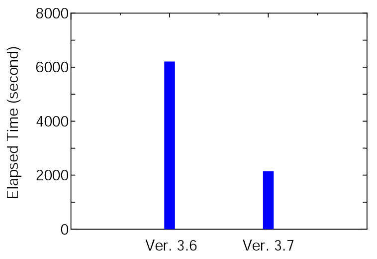
      where 128 MPI processes and 2 OpenMP threads on CRAY-XC30 were used for both the versions. It is found that Ver. 3.7 is about three times faster than Ver. 3.6 for the benchmark sets. The elapsed time for each input file can be confirmed from 'runtestL.result_xc30_v3.6' and 'runtestL.result_xc30' stored in 'work/large_example'.

    (3) ELPA based parallel eigensolver (supported by T.V.T. Duy and T. Ozaki)

      OpenMX Ver. 3.7 employs ELPA1 to solve the eigenvalue problem in the cluster and band calculations, which is a highly parallelized eigevalue solver. The eigenvalue solver enables us to perform geometry optimization for systems consisting of 1000 atoms if several hundreds processor cores are available. To demonstrate the capability, one can perform 'runtestL2' as follows:
           % mpirun -np 128 openmx -runtestL2 -nt 4
        
      Then, OpenMX will run with 7 test files, and compare calculated results with the reference results which are stored in 'work/large2_example'. The following is a result of 'runtestL2' performed using 128 MPI processes and 4 OpenMP threads on CRAY-XC30.

      1 large2_example/C1000.dat Elapsed time(s)= 1731.83 diff Utot= 0.000000002838 diff Force= 0.000000007504
      2 large2_example/Fe1000.dat Elapsed time(s)=21731.24 diff Utot= 0.000000010856 diff Force= 0.000000000580
      3 large2_example/GRA1024.dat Elapsed time(s)= 2245.67 diff Utot= 0.000000002291 diff Force= 0.000000015333
      4 large2_example/Ih-Ice1200.dat Elapsed time(s)= 952.84 diff Utot= 0.000000000031 diff Force= 0.000000000213
      5 large2_example/Pt500.dat Elapsed time(s)= 6831.16 diff Utot= 0.000000002285 diff Force= 0.000000004010
      6 large2_example/R-TiO2-1050.dat Elapsed time(s)= 2259.97 diff Utot= 0.000000000106 diff Force= 0.000000001249
      7 large2_example/Si1000.dat Elapsed time(s)= 1655.25 diff Utot= 0.000000001615 diff Force= 0.000000005764
      Total elapsed time (s) 37407.95

      The quality of all the calculations is at a level of production run where double valence plus a single polarization functions are allocated to each atom as basis functions. Except for 'Pt500.dat', all the systems include more than 1000 atoms, where the last number of the file name implies the number of atoms for each system, and the elapsed time implies that geometry optimization for systems consisting of 1000 atoms is possible if several hundred processor cores are available. It is noted that the parallel eigenvalue solver introduced in OpenMX Ver. 3.7 is not exactly the same as ELPA1 distributed in here. Since we found that the original ELPA1 tends to encounter a numerical instability on some platforms, we modified ELPA1 to make it stabilized. The original parallel eigenvalue solver used in OpenMX Ver. 3.6 is also available by the following keyword:

          scf.eigen.lib    elpa1   # elpa1|lapack, default=elpa1
       
      One can choose either 'elpa1' or 'lapack' depending on computational environment. The default is 'elpa1'. Due to the introduction of the ELPA based eigenvalue solver, users are requested to specify a FORTRAN compiler.

      More information can be found in here and here.

    (4) Massive parallelization of the O(N) Krylov subspace method (supported by T.V.T. Duy and T. Ozaki)

      The O(N) Krylov subspace method is massively parallelized to realize large-scale calculations of systems including a hundred thousand atoms. A new parallel algorithm and data structure have been developed so that the parallel execution can be possible on massively parallel computers consisting of more than a hundred thousand CPU cores and the data usage can be inversely proportional to the number of MPI processes. The details of the implementation can be found in arXiv:1209.4506 and arXiv:1302.6189v1. As a benchmark calculation, the parallel efficiency for the hybrid parallelization on the K-computer is shown below:
      Bench_K

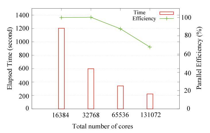
      where the diamond structure consisting of 131072 carbon atoms was considered as a benchmark system, and eight OpenMP threads were used for all the cases. The parallel efficiency is about 68 % using 131072 cores by taking the case with 16384 cores as a reference. No additional keyword is introduced for the development. The new development has been already applied to two large-scale systems, resulting in two papers: J. Chem. Phys. 136, 134101 (2012) and Modelling Simul. Mater. Sci. Eng. 21, 045012 (2013).

      Related information can be found in the manual.

    (5) Parallelization for k-point (supported by T. Ozaki)

      Up to and including Ver. 3.6, the number of MPI processes that users can utilize for the parallel calculations is limited up to the number of atoms in the system. OpenMX Ver. 3.7 does not have the limitation. Even if the number of MPI processes exceeds the number of atoms, the MPI parallelization is efficiently performed. The functionality may be useful especially for a calculation where the number of k-points is much larger than the number of atoms in the system. No additional keyword is introduced for the development.

      Related information can be found in here and here.

    (6) Parallelization for NEB (supported by Y. Kubota and F. Ishii)

      Although the default parallelization scheme for the NEB calculation works well in most cases, a memory shortage can be a serious problem when a small number of the MPI processes is used for large-scale systems. In the default MPI parallelization, the images are preferentially parallelized at first. When the number of MPI processes exceeds the number of images, the calculation of each image starts to be parallelized, where the memory usage starts to be parallelized as well. In this case, users may encounter a segmentation fault due to the memory shortage if many CPU cores are not available. To avoid such a situation, the following keyword is available.
          MD.NEB.Parallel.Number    3
         
      In this example, the calculations of every three images are parallelized at once where the MPI processes are classified to three groups and utilized for the parallelization of each image among the three images. In order to complete the calculations of all the images, the grouped calculations are repeated by floor[(the number of images)/(MD.NEB.Parallel.Number)] times. The scheme may be useful for the NEB calculation of a large-scale system. If the keyword is not specified in your input file, the default parallelization scheme is employed. Related information can be found in the manual.
    (7) Compatibility with the database Ver. 2013 of VPS and PAO (supported by T. Ozaki)

      The database Ver. 2013 of VPS and PAO was tested with OpenMX Ver. 3.7. One can reproduce the same result shown in the database using input files provided on the same web site. Some more information can be found in the manual.
    (8) Other changes are listed below:

      Multi-heat bath molecular dynamics: manual.
      Fully three dimensional parallelization: manual.
      Analysis of memory usage: manual.
      Output of large-sized files in binary mode: manual.
    (9) Bugs fixed

      Minor bugs in OpenMX Ver. 3.6 were fixed.
    (10) Manual revised

      The manual of OpenMX was revised.

30/Apr./2013

Database Ver. 2013 of optimized VPS and PAO was released.

Fully relativistic pseudopotentials (VPS) and pseudo-atomic orbitals (PAO), generated by ADPACK Ver. 2.2, are released at database (2013). The pseudopotentials are generated by the Morrison, Bylander, and Kleinman (MBK) scheme (Phys. Rev. B 47, 6728 (1993)), while the pseudo-atomic orbitals are optimized by the variational optimization method (Phys. Rev. B. 67, 155108, (2003)). Based on the database (2011), we further optimized both the pseudopotentials and pseudo-atomic orbitals so that benchmark calculations can be close to the corresponding all electron calculations more than those of the database (2011). Since the results of the benchmark calculations and input files used for the calculations are also presented in the database, they are expected to be a good starting point when a user starts own calculations. The accuracy of the database (2013) was valiated by the delta factor proposed in arXiv:1204.2733v3. The mean delta factor of 71 elements is 1.538 meV/atom with the standard deviation of 1.423 meV/atom, which implies high accuracy of the database (2013). Users are strongly encouraged to use the new database due to the high accuracy. The use of the old databases is never recommended anymore.

14/Nov./2011

The patch (Ver.3.6.1) of OpenMX Ver. 3.6 was released.

A patch 3.6.1 to OpenMX Ver. 3.6 was released at patch3.6.1.tar.gz.
After releasing OpenMX Ver. 3.6, we have noticed that some of routines are very sensitive to the compiler option used especially for Intel compiler. To address the issue, we have decided to use a pragma command, that is,
 #pragma optimization_level 1 
Then, the optimization level is always set to 1 for those routines without depending on the optimization level user defines. The other purposes of the patch can be found at README.txt.

Thank you very much for your cooperation in advance.

10/Nov./2011

OpenMX Ver 3.6 (with user's manual) was released.

The main features of the modifications are as follows:
    (1) Numerically exact low-order scaling method (supported by T. Ozaki)

      A numerically exact low-order scaling method for diagonalization is supported for large-scale calculations. The computational effort of the method scales as O(N(logN)2 ), O(N2), and O(N7/3) for one, two, and three dimensional systems, respectively, where is the number of basis functions. The details of the implementation can be found in PRB 82, 075131 (2010). The usage of the functionality can be found in the manual.
    (2) Effective screening medium (ESM) method (supported by T. Ohwaki)

      The effective screening medium (ESM) method is available for calculations of charged or biased systems consisting of a slab. An isolated slab, charged slab, and a slab under an uniform electric field can be treated by introducing ESM as boundary condition for the Hartree potential. The original proposal is M. Otani and O. Sugino, Phys. Rev. B 73, 115407 (2006). The usage of the functionality can be found in the manual.
    (3) Nudged elastic band (NEB) method (supported by T. Ozaki)

    (4) STM image by the Tersoff-Hamann scheme (supported by T. Ozaki)

      Scanning tunneling microscope (STM) image can be obtained by the Tersoff-Hamann scheme. The usage of the functionality can be found in the manual.
    (5) DFT-D2 method for vdW interaction (supported by Y. Okuno, P.P. Bell, and T. Ozaki)

      The DFT-D2 method by Grimme (J. Comput. Chem. 27, 1787 (2006)) is supported to include a vdW interaction. The usage of the functionality can be found in the manual.
    (6) Compatibility with the database Ver. 2011 of VPS and PAO (supported by T. Ozaki)

      The database Ver. 2011 of VPS and PAO was tested with OpenMX Ver. 3.6. One can reproduce the same result shown in the database using input files provided on the same web site. Some more information can be found in the manual.
    (7) Improvement of orbital optimization method (supported by T. Ozaki)

      The convergence of orbital optimization method is improved by employing quasi Newton type optimizers. The usage of the functionality can be found in the manual.
    (8) Fermi surface (supported by T. Ozaki)

      A bxsf file is provided to analyze Fermi surface with XCrySDen. The usage of the functionality can be found in the manual.
    (9) XSF files for the NC-DFT calculation (supported by T. Ozaki)

      XSF files are provided to analyze vector field for the NC-DFT calculations. The details can be found in the manual.
    (10) Calculation of 'Energy vs. lattice constant' (supported by T. Ozaki)

      An automatic calculation of 'Energy vs. lattice constant' is supported. The usage of the functionality can be found in the manual.
    (11) On-the-fly control of SCF mixing parameters (supported by M. Ohfuchi and T. Ozaki)

      It is possible to control SCF mixing parameters during SCF iteration. The usage of the functionality can be found in the manual.
    (12) Easy use of empty atom (supported by T. Ozaki)

      The use of empty atom is simplified. One can easily put any basis funtions to any place. The usage of the functionality can be found in the manual.
    (13) Integrated (P)DOS (supported by K. Sawada)

      Integrated (P)DOS is supported as a functionality of DosMain. The usage of the functionality can be found in the manual.
    (14) Parallelization of jx (supported by F. Ishii)

      The code, jx, which calculates an effective exchange interaction parameter, is parallelized. The usage of the functionality can be found in the manual.
    (15) Automatic determination of Kerker factor (supported by T. Ozaki)

      If the keyword, scf.Kerker.factor, is not specified, then a proper value of the Kerker factor is automaticaly determined for a given system. The details of the functionality can be found in the manual.
    (16) User definition of atomic mass (supported by T. Ozaki)

      The user definition of atomic mass is supported. The details of the functionality can be found in the manual.
    (17) Bugs fixed

      Minor bugs in OpenMX Ver. 3.5 were fixed.
    (18) Manual revised

      The manual of OpenMX was revised.

29/Sep./2011

The patch (Ver.3.5.4) of OpenMX Ver. 3.5 was released.

A bug in XC_PBE.c was found. The program bug is due to an improper use of '#define' command, which may cause a little change in the total energy. The bug was fixed, and a patch is available at patch3.5.4.tar.gz.
The patch contains three files: TRAN_Set_CentOverlap.c, Cluster_DFT.c, and XC_PBE.c.
Thank you for your cooperation in advance.

28/Sep./2011

Database Ver. 2011 of optimized VPS and PAO was released.

Fully relativistic pseudopotentials (VPS) and pseudo-atomic orbitals (PAO), generated by ADPACK Ver. 2.2, are released at database Ver. 2011. The pseudopotentials are generated by the Morrison, Bylander, and Kleinman (MBK) scheme (Phys. Rev. B 47, 6728 (1993)), while the pseudo-atomic orbitals are optimized by the variational optimization method (Phys. Rev. B. 67, 155108, (2003)). The optimizations for both the pseudopotentials and pseudo-atomic orbitals were carefully performed so that benchmark calculations can be well compared to the corresponding all electron calculations. Since the results of the benchmark calculations and input files used for the calculations are also presented in the database, they are expected to be a good starting point when a user starts own calculations. Users are strongly encouraged to use the new database due to the high accuracy. The use of the old databases Vers. 2004 and 2006 is never recommended anymore.

28/Sep./2011

ADPACK Ver 2.2 (with user's manual) was released.

The main features of the modifications are as follows:
    (1) Morrison, Bylander, and Kleinman (MBK) pseudopotential

    A norm-conserving pseudopotential proposed by Morrison, Bylander, Kleinman (MBK) (Phys. Rev. B 47, 6728 (1993)) is supported by the following keyword:
         vps.type    MBK
     
    The MBK pseudopotential is a norm-conserving version of the Vanderbilt's ultrasoft pseudopotential (Phys. Rev. B 41, 7892 (1990)). The feature allows us to take multiple states with the same angular momentum quantum number into account for construction of a separable pseudopotential. Thus, it is guranteed that the MBK scheme is more accurate than the other norm-conserving schemes when semi-core states are included in the construction of pseudopotential.
    (2) Finite element method (FEM) for atomic LDA and Hartree-Fock calculations

    A highly accurate finite element method (FEM) (Comp. Phys. Comm. 182, 1245 (2011)) is available for all electron calculations within LDA by Vosko, Wilk, and Nusair and the Hartree-Fock scheme. In the calculations, spherical charge distribution and spherical potential are assumed for the Schrodinger equation. The FEM calculation is not supported for the Dirac equation. The details for usage is found in the manual, and technical descriptions of implementation is found in a paper.
    (3) Bugs fixed

      Minor bugs in ADPACK Ver. 2.1 were fixed.
    (4) Manual revised

      The manual of ADPACK was revised.

30/Aug./2011

The patch (Ver.3.5.2) of OpenMX Ver. 3.5

A bug in TRAN_Set_CentOverlap.c was reported by R. Miceli. The program bug is due to an improper access to an array, which may cause a segmention fault. The bug was fixed, and a patch is available at patch3.5.2.tar.gz .
The patch contains two files: TRAN_Set_CentOverlap.c and Cluster_DFT.c.
Thank you for your cooperation in advance.

13/May/2011

The patch (Ver.3.5.1) of OpenMX Ver. 3.5

A bug in Cluster_DFT.c was reported by R. Miceli. The program bug is due to an improper treatment for rounding down in division of integer numbers. For relatively large-scale systems, it is possible OpenMX to encounter a segmention fault. The bug was fixed, and a patch is available at patch3.5.1.tar.gz . The patch contains one file: Cluster_DFT.c.
Thank you for your cooperation in advance.

10/Sep./2009

OpenMX Ver 3.5 (with user's manual) was released.

The main features of the modifications are as follows:

    (1) Electronic transport calculations (supported by T. Ozaki and H. Kino)

      Electronic transport properties of molecules, nano-wires, and bulks such as superlattice structures can be calculated based on a non-equilibrium Green function (NEGF) method within the collinear DFT. The features and capabilities are listed below:

        1. SCF calculation of system with two leads under zero and a finite bias voltages
        2. SCF calculation under gate bias voltage
        3. Compatible with the LDA+U method
        4. Spin-dependent transmission and current
        5. k-resolved transmission and current along perpendicular to the current axis
        6. Calculation of current-voltage curve
        7. Accurate and efficient contour integration scheme
        8. Interpolation of the effect by the bias voltage
        9. Quick calculation for periodic systems under zero bias

      The details of the implementation can be found in PRB 81, 035116 (2010) | arXiv:0908.4142 . The usage of the functionalities can be found in the manual.

    (2) Construction of maximally localized wannier functions (supported by H. Weng and T. Ozaki)


    (3) Bugs fixed

      Minor bugs in OpenMX Ver. 3.4 were fixed.

    (4) Manual revised

      The manual of OpenMX was revised.

17/Mar./2009

The patch (Ver.3.4.4) of OpenMX Ver. 3.4

The size of the long integer is 8 bites in a 64 bit processor, AMD Shanghai, while the size is 4 bites for machines we tested before. The change of size of the long integer may cause a segmentation fault in the subroutine, truncation.c. The bugs were fixed and a new patch of Ver.3.4 was released at patch3.4.4.tar.gz . The patch contains four files: SetPara_DFT.c, Set_Aden_Grid.c, Set_OLP_Kin.c, and truncation.c. Thank you for your cooperation in advance.

04/Dec./2008

The patch (Ver.3.4.3) of OpenMX Ver. 3.4

Even though the patch3.4.2 is applied to OpenMX ver.3.4, it is found that in some case the empty atom is not treated properly. Also, OpenMX ver.3.4 may encounter segmentation faults in the calculation of a single isolated atom. The bugs were fixed and a new patch of Ver.3.4 was released at patch3.4.3.tar.gz . The patch contains three files: SetPara_DFT.c, Set_Aden_Grid.c, and Set_OLP_Kin.c. Thank you for your cooperation in advance.

27/Nov./2008

The patch (Ver.3.4.2) of OpenMX Ver. 3.4

Although the patch3.4.1 was released in 06/Nov./2008, the patch was not compatible with Ver.3.4 of OpenMX because of the insufficient testing for compatibility. The bug was fixed and a new patch of Ver.3.4 was released at patch3.4.2.tar.gz . The patch contains two files: SetPara_DFT.c and Set_Aden_Grid.c. Thank you for your cooperation in advance.

06/Nov./2008

The patch (Ver.3.4.1) of OpenMX Ver. 3.4

As Mr. Jeong pointed out in the forum, the empty atom is not treated properly in OpenMX Ver.3.4. The bug was fixed and the patch of Ver.3.4 was released at patch3.4.1.tar.gz . The patch contains two files: SetPara_DFT.c and Set_Aden_Grid.c. Thank you for your cooperation in advance.

23/June/2008

OpenMX Ver 3.4 (with user's manual) was released.

The main features of the modifications are as follows:

    (1) OpenMP/MPI hybrid parallelization

      The OpenMP/MPI hybrid parallel execution can be performed by
          % mpirun -np 32 openmx DIA512-1.dat -nt 4 > dia512-1.std &
        
      where '-nt' means the number of threads in each process managed by MPI. If '-nt' is not specified, then the number of threads is set 1, which corresponds to the pure MPI parallelization. For the installation, please see the manual.

      Figure shows the elapsed time (sec.) and the required memory size (Mbyte) per node in calculations for the O(N) Krylov subspace, the cluster, and the band methods, respectively, where the number of cores is given by the number of processes by MPI times the number of threads by OpenMP. As you can see, the hybrid parallelization using 2 or 4 threads is not fast in the region using the smaller number of processes. However, the hybrid parallelization gives us the shortest elapsed time eventually as the number of processes increases. This behavior may be understood as follows: in the region using the smaller number of processes the required memory size is large enough so that cash miss easily happens. This may lead to considerable communication between processor and memory via bus. So, in the region using the smaller number of processes, the bus becomes a bottle neck in terms of elapsed time. On the other hand, in the region using the large number of processes, the required memory size is small enough that most of data can be stored in the cashes. So, the efficiency in OpenMP parallelization can be recovered. In this case, the hybrid parallelization can obtain both the benefits of MPI and OpenMP. Thus, the hybrid parallelization should be eventually efficient as the number of processes increases. In fact, our benchmark calculation may be the case. Also, it should be emphasized that the required memory size per node can be largely reduced in the hybrid parallelization in OpenMX as shown in the Figure.

      Figure: The elapsed time (sec.) and the required memory size (Mbyte) per node in calculations for (a) and (d) the O(N) Krylov subspace, (b) and (e) the cluster, and (c) and (f) the band methods, respectively, where the number of cores is given by the number of processes by MPI times the number of threads by OpenMP. The machine used is an Opteron cluster consisting of two dual core AMD Opteron (tm) processors 2218, 2.6 GHz, with 8 Gbyte memory per node. Those nodes are connected with Gbit ether network. The input files used for those calculations are DIA512-1.dat, Mn12.dat, and DIA64_Band.dat for the O(N) Krylov subspace, the cluster, and the band methods, respectively. They can be found in the directory 'work'.
      \begin{figure}\begin{center}
   \epsfig{file=hybrid-para.eps,width=9.37cm} \end{center} \end{figure}

    (2) Virtual atom with fractional nuclear charge

      It is possible to treat a virtual atom with fractional nuclear charge by using a pseudopotential with the corresponding fractional nuclear charge. The pseudopotential for the virtual atom can be generated by ADPACK. The relevant keywords in ADPACK are given by
           AtomSpecies            6.2
           total.electron         6.2
           valence.electron       4.2 
           <ocupied.electrons 
            1   2.0
            2   2.0  2.2
           ocupied.electrons>
        
      The above example is for a virtual atom on the way of carbon and nitrogen atoms. Also, it is noted that basis functions for the pseudopotential of the virtual atom must be generated for the virtual atom with the same fractional nuclear charge, since the atomic charge density stored in *.pao is used to make the neutral atom potential. As an illustration, the DOS of C$_{7.8}$N$_{0.2}$ calculated using the method is shown in Fig. The input file is DIA8-VA.dat which can be found in the directory, work. In the calculation, one of eight carbon atoms in the unit cell was replaced by a virtual atom with an effective nuclear charge of 4.2, which corresponds to a stoichiometric compound of C$_{7.8}$N$_{0.2}$.
      Figure: Density of states (DOS) of C$_{7.8}$N$_{0.2}$ calculated with a pseudopotential of the virtual atom. The input file used for the calculation is DIA8-VA.dat which can be found in the directory, work.
      \begin{figure}\begin{center}
  \epsfig{file=dia8-va.eps,width=13.0cm} \end{center} \end{figure}


    (3) Input file for the restart

      An input file, *.dat#, is generated at every MD step for the restart calculation with the final structure and the same 'Grid_Origin' explained in the Sec. 'Fixing the relative position of regular grid'. Using the file, *.dat#, it can be possible to continue MD calculations and geometry optimization from the last step.

    (4) Automatic running test with large-scale systems

      In some cases, one may want to know machine performance for more time consuming calculations. For this purpose, an automatic running test with relatively large-scale systems can be performed by

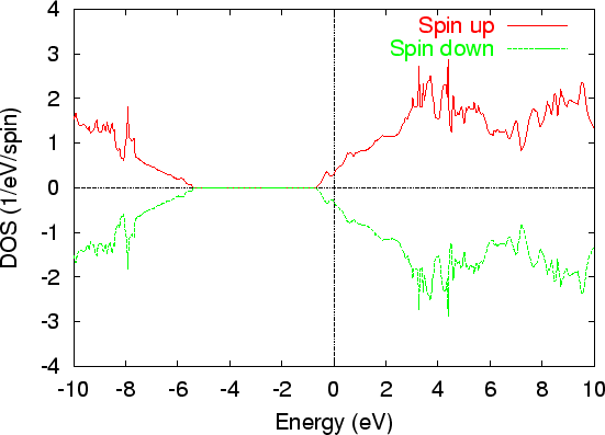
      For the serial running

           % ./openmx -runtestL
        
      For the MPI parallel running
           % mpirun -np 4 openmx -runtestL
        
      For the OpenMP/MPI parallel running
           % mpirun -np 4 openmx -runtestL -nt 1
        
      Then, OpenMX will run with 20 test files, and compare calculated results with the reference results which are stored in 'work/large_example'. The comparison (absolute difference in the total energy and force) is stored in a file 'runtestL.result' in the directory 'work'. Since the automatic running test requires considerable memory size, you may encounter a segmentation fault on computational environment with small memory. Also it is noted that the total elapsed time is more than 1 day even using 40 cores.

    (5) Re-normalization of atomic charge density

      After PAO files are read, atomic charge density is re-normalized by OpenMX. This causes a little energy change compared to OpenMX Ver. 3.3. So, it is better to avoid directly comparing the total energies calculated by Vers. 3.3 and 3.4.

    (6) Bugs fixed

      Minor bugs in OpenMX Ver. 3.3 were fixed.

    (7) Manual revised

      The manual of OpenMX was revised.

20/June/2008

ADPACK Ver 2.1 (with user's manual) was released.

The main features of the modifications are as follows:

    (1) Treatment of virtual atom with fractional nuclear charge

    It is possible to generate pseudopotentials and basis functions for a virtual atom with fractional nuclear charge. The relevant keywords in ADPACK are given by
         AtomSpecies            6.2
         total.electron         6.2
         valence.electron       4.2 
         <ocupied.electrons 
          1   2.0
          2   2.0  2.2
         ocupied.electrons>
     
    The above example is for a virtual atom on the way of carbon and nitrogen atoms. By just controling the above keywords, you can easily generate pseudopotentials and basis functions for virtual atoms. When you use those in OpenMX as input data, no specification by keywords is required. Please make sure that only OpenMX Ver. 3.4 or later accepts the pseudopotentials and the basis functions for the virtual atoms. Also, it is noted that basis functions for the pseudopotential of the virtual atom must be generated for the virtual atom with the same fractional nuclear charge, since the atomic charge density stored in *.pao is used to make the neutral atom potential in OpenMX.

    (2) Bugs fixed

      Minor bugs in ADPACK Ver. 2.0 were fixed.

    (3) Manual revised

      The manual of ADPACK was revised.

25/Sep./2007

A patch of OpenMX Ver. 3.3

As Dr. Gusso pointed out, OpenMX Ver.3.3 encounters segmentation fault in case of "scf.ProExpn.VNA=off". The bug was fixed and the patch of Ver.3.3 was released at patch3.3.1.tar.gz . The patch contains three files: Set_Vpot.c, Total_Energy.c, and openmx_common.h.
Thank you for your cooperation in advance.

20/Aug./2007

Release of Technical Notes

Technical notes on OpenMX and ADPACK have been released at here.

30/July/2007

OpenMX Ver 3.3 was released.

Three methods for geometry optimization have been newly implemented, while the manual of the version 3.3 is not released. Please find distinct features of the modifications below:

    (1) Implementation of three geomergy optimizers (EF, RF, and BFGS methods) (supported by Dr. H. Weng and TO)

      Three methods for geometry optimization have been newly implemented in OpenMX3.3. They are the eigenvector following (EF) method, (J. Baker, J. Comput. Chem. 7, 385 (1986)), the rational function (RF) method (A. Banerjee et al., J. Phys. Chem. 89, 52 (1986)), and the Broyden-Fletcher-Goldfarb-Shanno (BFGS) method (C. G. Broyden, J. Inst. Math. Appl. 6, 76 (1970); R. Fletcher, Comput. J. 13, 317 (1970); D. Goldrarb, Math. Comp. 24, 23 (1970); D. F. Shanno, Math. Comp. 24, 647 (1970)) implemented in the cartesian coodinate. In the EF and RF methods, the approximate Hessian is updated by the BFGS method. Thus, five geometry optimizers, Opt, DIIS, EF, RF, and BFGS, are available in OpenMX3.3, which can be specified by "MD.Type". The relevant keywords are listed below:
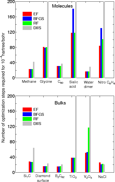
      MD.Type                     EF         # Opt|DIIS|BFGS|RF|EF
      MD.Opt.DIIS.History          3         # default=3
      MD.Opt.StartDIIS             5         # default=5
      MD.Opt.EveryDIIS            200        # default=200
      MD.maxIter                  100        # default=1
      MD.Opt.criterion          1.0e-4       # default=0.0003 (Hartree/bohr)
       
      Since the usages of these keywords are same as in the previous version 3.2, you can find the details in the manual of the previous version 3.2. The initial step in the optimization is automatically tuned by monitoring the maximum force in the initial structure, while it was specified by the keyword "MD.Initial.MaxStep" in the previous version 3.2 (the keyword "MD.Initial.MaxStep" is not available in OpenMX3.3). As shown in the figure which shows the number of geometry steps to achieve the maximum force of below 0.0001 hartree/bohr in molecules and bulks, in most cases the EF method seems to be the most robust and efficient scheme, while the RF method also shows a good performance.


      Thus, it is recommented to try the EF method firstly. For your convenience, the input files and out files used in the calculations shown in the figure can be found in "openmx3.3/work/geoopt_example".

    (2) Bugs fixed

      Several bugs in OpenMX Ver. 3.2 were fixed.

02/July/2007

A patch #4 of OpenMX Ver. 3.2

Since a file 'DFT.c' in the patch #3 of OpenMX Ver. 3.2 seems to be broken during the file transfer, the patch #4 of OpenMX Ver. 3.2 was released. Please replace the routines by patch3.2.4.tar.gz . The patch contains all the corrected subroutines in patch3.2.1 and patch3.2.2. Sorry for the frequent releases, and thank you for your cooperation in advance.

28/June/2007

A patch #3 of OpenMX Ver. 3.2

In the non-collinear calculation, the evaluation of the Voronoi charge was improper, and the calculation became unstable as the spin angle approaches to 90 deg of 'theta' (the first angle). The relevant bugs were fixed in several routines. Please replace the routines by patch3.2.3.tar.gz . The patch contains all the corrected subroutines in patch3.2.1 and patch3.2.2. Thank you for your cooperation in advance.

22/Apr./2007

A patch #2 of OpenMX Ver. 3.2

As Dr. JessK reported (Thanks to Dr. Jessk), OpenMX3.2 with the patch which was released at 13/Apr./2007 fails to calculate 'CO.dat' in the runtest. The relevant bug was fixed in DFT.c.
Please replace the routine by patch3.2.2.tar.gz . The patch contains all the corrected subroutines including those released at 13/Apr./2007. Thank you for your cooperation in advance.

13/Apr./2007

A patch #1 of OpenMX Ver. 3.2

After the release of Ver.3.2, a couple of users reported possible bugs (Thanks to them). The relevant bugs were fixed in four rouintes as follows:

'DFT.c'
A bug that the restart does not work properly in the LDA+U method was fixed.

'MD_pac.c'
A bug that a keyword 'MD.Opt.StartDIIS' does not work properly was fixed.

'EulerAngle_Spin.c' and 'Voronoi_Charge.c'
In the non-collinear caculation, the calculation of Voronoi charge is improper in Ver.3.2 as the spin angle approches to 90 (Deg). The bug was fixed.

Please replace these routines by patch3.2.1.tar.gz . Thank you for your cooperation in advance.

01/Apr./2007

OpenMX Ver 3.2 (with user's manual) was released.

The main features of the modifications are as follows:

    (1) Improvement of parallelization

      The parallelization for the cluster and band calculations was improved for the large-scale calculations. In the cluster calculation, a double parallelization is made for two loops: spin multiplicity and eigenstates, where the spin multiplicity means one, two, and one for spin-unpolaized, spin-polarized, and non-collinear calculations, respectively. The priority of parallelization is in order of spin multiplicity and eigenstates. In the band calculation, a triple parallelization is made for three loops: spin multiplicity, k-points, and eigenstates. The priority of parallelization is in order of spin multiplicity, k-points, and eigenstates. In addition, when the number of processors used in the parallelization exceeds (spin multiplicity)(the number of k-points), OpenMX uses an efficient way in which finding the Fermi level and calculating the density matrix are performed by just one diagonalization at each k-point. For the other cases, twice diagonalizations are performed at each k-point for saving the size of used memory in which the second diagonalization is performed to calculate the density matrix after finding the Fermi level. As a result, OpenMX Ver.3.2 becomes much faster than Ver. 3.1 for these parallel calculations. There is no additional keyword for this improvement. The details and test calculations can be found in the secion 'Parallelization' in the manual.

    (2) Extrapolation of charge density

      A charge extrapolation scheme (T. A. Arias, M. C. Payne, and J. D. Joannopoulos, PRB 45, 1538 (1992); D. Alfe, Comp. Phys. Commun. 118, 32 (1999).) was implemented to estimate a good input charge density for molecular dynamic simulations (MD) and geometry optimizations. The initial input charge density at every MD step is estimated by the extrapolation scheme using the self-consistent charge at the previous four MD steps. There is no additional keyword for this improvement.

    (3) Parallell calculation of electronic polarization (supported by Dr. F.Ishii)

      The calculation of electronic polarization by the post-processing code 'polB' has been parallelized using MPI. The parallelization allows us to apply the code to larger-scale systems compared to before.

    (4) As for the total energy

      Since some of routines were optimized for efficiency of calculations, and default values for several parameters have been changed, the total energy calculated by OpenMX Ver. 3.2 can be different from that by Ver. 3.1.

    (5) Reducing the memory requirement

      The memory used is reduced by optimizing the allocation of work arrays. In addition, two large arrays (DS_VNA and Orbs_Grid) are allocated in single-precision floating point. Since the type of floating point is specified in 'openmx_common.h', one can easily change the type of floating point. The relavant lines in 'openmx_common.h' are
      typedef float     Type_DS_VNA;          /* type of DS_VNA */
      #define MPI_Type_DS_VNA  MPI_FLOAT      /* type of DS_VNA */
      
      typedef float     Type_Orbs_Grid;       /* type of Orbs_Grid */
      #define MPI_Type_Orbs_Grid  MPI_FLOAT   /* type of Orbs_Grid */
       
      By changing 'float' and 'MPI_FLOAT' into 'double' and 'MPI_DOUBLE', it is possible to allocate them in double-precision floating point if you like it.

    (6) Change of an option name in the compilation

      The name of an option for 'CC' in the makefile was changed from '-Dbraswrap' to '-Dblaswrap'.

    (7) Bugs fixed

      Minor bugs in OpenMX Ver. 3.1 were fixed.

    (8) Manual revised

      The manual of OpenMX was revised.

01/Apr./2007

ADPACK Ver 2.0 (with user's manual) was released.

The main features of the modifications are as follows:

    (1) Pseudopotential generation for unbound states


    (2) Enhancement or depletion of a spin-orbit coupling

      To study the effect of a spin-orbit coupling, it is possible to generate a pseudopotential with a larger or smaller spin-orbit coupling compared to that in a real atom. The scaling factors can be specified to each angular momentum quantum number by the following keyword:
         <SO.factor
          0  1.0
          1  0.5
          2  2.0 
         SO.factor>
       
      The beginning of the description must be <SO.factor, and the last of the description must be SO.factor>. The number in the first column corresponds to that in the keyword 'pseudo.NandL', and a scaling factor is given for each pseudopotential by the second column, where '1.0' corresponds to the spin-orbit coupling in a real atom. One can control the strength of spin-orbit coupling by changing the scaling factor.

    (3) Stabilization of all electron calculations for heavy atoms

      All electron calculations for heavy atoms can be improved to increase the numerical stability. There is no additional keyword for this revision.

    (4) Bugs fixed

      Minor bugs in ADPACK Ver. 1.8 were fixed.

    (5) Manual revised

      The manual of ADPACK was revised.

01/Apr./2007

Renewal of the website

The website has been updated largely and the URL of the top page has been changed.

17/Nov./2006

Bugs in Total_Energy.c of OpenMX Ver. 3.1

A bug was fixed in a routine 'Total_Energy.c' of OpenMX Ver. 3.1. In the non-collinear calculation, there is a bug in evaluation of the contribution of the non-local potentials to the total energy (Thanks Dr. Hosik Lee at SNU for reporting the bug). Please replace this routine by Total_Energy.c . Thank you for your cooperation in advance.

13/Nov./2006

Bugs in DFT.c of OpenMX Ver. 3.1

A bug was fixed in a routine 'DFT.c' of OpenMX Ver. 3.1. When the k-space mixing methods (Kerker and RMM-DIISK) are used, the restarting of job with the restarting file did not work properly in the version 3.1. Please replace this routine by DFT.c . Thank you for your cooperation in advance.

4/Nov./2006

OpenMX Ver 3.1 was released.

Since the manual of the version 3.1 is not released, please find distinct features of the modifications below:

    (1) Analysis of difference charge density induced by the interaction

      The redistribution of charge (spin) density induced by the interaction between two systems A and B can be analyzed by the following procedure:

      (i) calculate the composite system consisting of A and B

      Then, you will have a cube file for charge (spin) density. Let it 'AB.cube'. Also, you will find 'Grid_Origin' in the standard output which gives x-, y-, and z-components of the origin of the regular grid as:
             Grid_Origin  xxx  yyy  zzz
            
      The values will be used in the following calculations (ii) and (iii).

      (ii) calculate the system A

      This calculation must be performed by the same calculation condition with the same unit cell as in the composite system consisting of A and B. Also, the coordinates of the system A must be the same as in the calculation (i). To use the same origin as in the calculaiton (i) rather than the use of an automatically determined origin, you have to include the following keyword in your input file.
              scf.fixed.grid  xxx  yyy  zzz
             
      where 'xxx yyy zzz' is the coordinate of the origin you got in the calculation (i). Then, you will have a cube file for charge (spin) density. Let it 'A.cube'.

      (iii) calculate the system B

      As well as the calculation (ii), this calculation must be performed by the same calculation condition with the same unit cell as in the composite system consisting of A and B. Also, the coordinates of the system B must be the same as in the calculation (i). To use the same origin as in the calculaiton (i) rather than the use of an automatically determined origin, you have to include the following keyword in your input file.
              scf.fixed.grid  xxx  yyy  zzz
             
      where 'xxx yyy zzz' is the coordinate of the origin you got in the calculation (i). Then, you will have a cube file for charge (spin) density. Let it 'B.cube'.

      (iv) compile two codes

      comile two codes as follows:
            % gcc diff_gcube.c -lm -o diff_gcube
            % gcc add_gcube.c -lm -o add_gcube
            
      (v) generate a cube file for differece charge (spin) density

      First, generate a cube file for the superposition of two charge (spin) densities of the systems A and B by
             % ./add_gcube A.cube B.cube A_B.cube
             
      The file 'A_B.cube' is the cube file for the superposition of charge (spin) density of two isolated systems. Then, you can generate a cube file for the difference charge (spin) density induced by the interaction as follows:
             % ./diff_gcube AB.cube A_B.cube dAB.cube
             
      The file 'dAB.cube' is the cube file for the difference charge (spin) density induced by the interaction, where the difference means (AB - A_B).

    (2) Specification of the path to the VPS and PAO

      The path to the VPS and PAO directories can be specified in your input file by the following keyword:
          DATA.PATH    ../DFT_DATA2006/    # default=../DFT_DATA/
             
      Both the absolute and relative specifications are available.

    (3) Gaussian DOS for bulk systems

      Since the calculation of density of states (DOS) of a large-scale system with a lot of k-points requires a considerable memory size, the post-processing code 'DosMain' for genenerating the partial and total DOS tends to suffer from a segmentation fault. For such a case, a Gaussian DOS scheme is available in which the partial DOS is calculated by the Gaussian broadening method in the OpenMX on-the fly calculation and the information of wave functions is not stored in the file '*.Dos.vec'. Since this scheme does not require a large size of memory, it can be used to calculate DOS of large-scale systems. Then, you can specify the following keywords in your input file.
             DosGauss.fileout      on       # default=off, on|off
             DosGauss.Num.Mesh    200       # default=200
             DosGauss.Width       0.2       # default=0.2 (eV)
            
      When you use the scheme, specify 'on' for the keyword 'DosGauss.fileout'. And the keyword 'DosGauss.Num.Mesh' gives the number of partitioning for the energy range specified by the keyword 'Dos.Erange'. The keyword 'DosGauss.Width' gives the width, a, of the Gaussian exp(-(E/a)^2). The keyword 'DosGauss.fileout' and the keyword 'Dos.fileout' are mutually exclusive. Therefore, when you use the scheme the keyword, 'Dos.fileout' must be 'off' as follows:
             Dos.fileout         off       # on|off, default=off
            
      Also, the following two keywords are valid for both the keywords 'Dos.fileout' and 'DosGauss.file'.
             Dos.Erange      -20.0  20.0   # default=-20 20 
             Dos.Kgrid          5 5 5      # default=Kgrid1 Kgrid2 Kgrid3
            
      It should be noted that the keyword 'DosGauss.fileout' generates only the Gaussian broadening DOS, which means that the DOS by the tetrahedron method cannot be calculated by the keyword 'DosGauss.fileout'.

    (4) Acceleration of calculation of electronic polarization (supported by Dr. F.Ishii)

      The calculation of electronic polarization by the post-processing code 'polB' is accelerated by eliminating the calculation of overlap matrix elements associated with unoccupied states.

    (5) Zeeman term for spin magnetic moment

      The Zeeman term for spin magnetic moment is available as an interaction with a uniform magnetic field by the following keywords:
            scf.NC.Zeeman.Spin           on        # on|off, default=off
            scf.NC.Mag.Field.Spin      1.0e+3      # default=0.0(Tesla) 
            
      When you include the Zeeman term for spin magnetic moment, switch on the keyword 'scf.NC.Zeeman.Spin'. The magnitude of the uniform magnetic field can be specified by the keyword 'scf.NC.Mag.Field.Spin' in units of Tesla. Moreover, we extend the scheme as a constraint scheme in which the direction of the magnetic field can be different from each atomic site atom by atom. Then, the direction of magnetic field for spin magnetic moment can be controlled, for example, by the keyword 'Atoms.SpeciesAndCoordinates':
        <Atoms.SpeciesAndCoordinates           
         1  Sc  0.000  0.000  0.000   6.6 4.4  10.0 50.0  160.0 20.0  1  on
         2  Sc  2.000  0.000  0.000   6.6 4.4  80.0 50.0  160.0 20.0  1  on
        Atoms.SpeciesAndCoordinates>
        
      The 8th and 9th columns give the Euler angles, theta and phi, in order to specify the magnetic field for spin magnetic moment. The 12th column is a switch to the constraint. '1' means that the constraint is applied, and '0' no constraint. Since for each atomic site a different direction of the magnetic field can be applied, this scheme provides a way of studying non-collinear spin configuration. It is noted that the keyword 'scf.NC.Zeeman.Spin' and the keyword 'scf.Constraint.NC.Spin' are mutually exclusive. Therefore, when 'scf.NC.Zeeman.Spin' is 'on', the keyword 'scf.Constraint.NC.Spin' must be switched off as follows:
            scf.Constraint.NC.Spin       off       # on|off, default=off
             
    (6) Zeeman term for orbital magnetic moment

      The Zeeman term for orbital magnetic moment is available as an interaction with a uniform magnetic field by the following keywords:
            scf.NC.Zeeman.Orbital        on        # on|off, default=off
            scf.NC.Mag.Field.Orbital   1.0e+3      # default=0.0(Tesla) 
            
      When you include the Zeeman term for orbital magnetic moment, switch on the keyword 'scf.NC.Zeeman.Orbital'. The magnitude of the uniform magnetic field can be specified by the keyword 'scf.NC.Mag.Field.Orbital' in units of Tesla. Moreover, we extend the scheme as a constraint scheme in which the direction of the magnetic field can be different from each atomic site atom by atom. Then, the direction of magnetic field for orbital magnetic moment can be controlled, for example, by the keyword 'Atoms.SpeciesAndCoordinates':
        <Atoms.SpeciesAndCoordinates           
         1  Sc  0.000  0.000  0.000   6.6 4.4  10.0 50.0  160.0 20.0  1  on
         2  Sc  2.000  0.000  0.000   6.6 4.4  80.0 50.0  160.0 20.0  1  on
        Atoms.SpeciesAndCoordinates>
        
      The 10th and 11th columns give the Euler angles, theta and phi, in order to specify the magnetic field for orbital magnetic moment. The 12th column is a switch to the constraint. '1' means that the constraint is applied, and '0' no constraint. Since for each atomic site a different direction of the magnetic field can be applied, this scheme provides a way of studying non-collinear orbital configuration. Also, it is noted that the direction of magnetic field for orbital magnetic moment can be different from that for spin moment.

    (7) Change of the format for non-collinear calculations

      As explained above, for the non-collinear calculations the specification of the keyword 'Atoms.SpeciesAndCoordinates' has been changed as follows:
        <Atoms.SpeciesAndCoordinates           
         1  Sc  0.000  0.000  0.000   6.6 4.4  10.0 50.0  160.0 20.0  1  on
         2  Sc  2.000  0.000  0.000   6.6 4.4  80.0 50.0  160.0 20.0  1  on
        Atoms.SpeciesAndCoordinates>
        
      The specification of each column is listed as:
         1:    sequential serial number
         2:    species name
         3:    x-coordinate
         4:    y-coordinate
         5:    z-coordinate
         6:    initial occupation for up spin
         7:    initial occupation for down spin
         8:    Euler angle, theta, of the magnetic field for spin magnetic moment
         9:    Euler angle, phi, of the magnetic field for spin magnetic moment
               Also, the 8th and 9th are used to generate the initial non-collinear 
               spin charge distribution
        10:    the Euler angle, theta, of the magnetic field for orbital magnetic moment
        11:    the Euler angle, phi, of the magnetic field for orbital magnetic moment
        12:    switch for the constraint schemes specified by the keywords 
               'scf.Constraint.NC.Spin', 'scf.NC.Zeeman.Orbital' and 'scf.NC.Zeeman.Orbital'.
               '1' means that the constraint is applied, and '0' no constraint.
        13:    switch for enhancement of orbital polarization in the LDA+U method, 
               'on' means that the enhancement is made, 'off' no enhancement.
            
    (8) Constrained geometry optimization and molecular dynamics

      It is possible to separately fix the x-, y-, and z-coordinates of the atomic position to the initial position in your input file by the following keyword:
          <MD.Fixed.XYZ
            1  1 1 1
            2  1 0 0
          MD.Fixed.XYZ>
           
      The example is for a system consisting of two atoms. If you have N atoms, then you have to provide N-th rows in this specification. The 1st column is the same sequential number to spefify atom as in the specification of the keyword 'Atoms.SpeciesAndCoordinates'. The 2nd, 3rd, 4th columns are switchs for the x-, y-, z-coordinates. '1' means that the coordinate is fixed, and '0' relaxed. It should be noted that the definition of the switch is opposite compared to the previous constraint schemes. In above example, the x-, y-, z-coordinates of the atom '1' are fixed, only the x-coordinate of the atom '2' is fixed. The default setting is that all the coordinates are relaxed. The fixing of atomic positions are valid all the geometry optimizer and molecular dynamics schemes. So, the previous constraint schemes such as 'Constraint_DIIS' are replaced by a combination of the keyword 'MD.Fixed.XYZ' and the geometry optimizer and molecular dynamics schemes specified by the keyword 'MD.Type'. Then, the following schemes are now available for the keyword 'MD.Type'.
            NoMD
            Opt
            DIIS
            NVE
            NVT_VS
            NVT_NH
          
    (9) Initial velocity for molecular dynamics

      For molecular dynamics simulations, it is possible to provide the initial velocity of each atom by the following keyword:
        <MD.Init.Velocity
         1    3000.000  0.0  0.0
         2   -3000.000  0.0  0.0
        MD.Init.Velocity>
            
      The example is for a system consisting of two atoms. If you have N atoms, then you have to provide N-th rows in this specification. The 1st column is the same sequential number to spefify atom as in the specification of the keyword 'Atoms.SpeciesAndCoordinates'. The 2nd, 3rd, and 4th columns are x-, y-, and z-components of the velocity of each atom. The unit of the velocity is m/s. The keyword 'MD.Init.Velocity' is compatible with the keyword 'MD.Fixed.XYZ'.

    (10) Bugs fixed

      Minor bugs in OpenMX Ver. 3.0 were fixed.

04/June/2006

Database (2006) of PAO and VPS

Fully relativistic pseudopotentials (VPS) and pseudo-atomic orbitals (PAO) of elements (Z=1 to 103), generated by ADPACK2.0 (not released yet), are now available.

24/Mar./2006

Bugs in MD_pac.c of OpenMX Ver. 3.0

Bugs were fixed in a routine 'MD_pac.c' of OpenMX Ver. 3.0. If you perform the DIIS geometry optimization, please replace this routine by MD_pac.c . Thank you for your cooperation in advance.

20/Mar./2006

OpenMX Ver 3.0 (with user's manual) was released.

The main features of the modifications are as follows:

    (1) Fractional coordinate

      The fractional coordinate is also available by 'FRAC' for the key word 'Atoms.SpeciesAndCoordinates'. In this case, please specify the coordinates spanned by a, b, and c-axes given in 'Atoms.UnitVectors'.

    (2) Empty atom scheme

      It is possible to assign basis functions in any vacant region using an 'empty' atom. You will find the empty atom 'E' in the database (http://staff.aist.go.jp/t-ozaki/vps_pao). Using the basis functions and pseudopotential, though the pseudopotential is a flat zero potential, you can put the basis functions at any place independently of atomic position. The empty atom scheme enables us to treat a vacancy state and a nearly free electron state on metal surfaces within the LCAO method. For the details, see 'Section 8.3 Empty atom scheme' in the manual.

    (3) Stable DIIS geometry optimization

      A Stable DIIS geometry optimization is available by 'DIIS' for the keyword 'MD.Type' Then, you can control this scheme by two keywords:
              MD.Opt.DIIS.History      4       # default=4
              MD.Opt.StartDIIS         5       # default=5
            
      The keyword 'MD.Opt.DIIS.History' specifies the number of the previous steps to estimate an optimum structure which will give the minimum norm of forces used. The default value is 4. Also, the geometry optimization step which starts 'DIIS' is specified by the keyword 'MD.Opt.StartDIIS'. The geometry optimization steps before starting DIIS type methods is performed by the steepest decent method as in 'Opt'. The default value is 5. For the details, see 'Section 13 Geometry optimization' in the manual.

    (4) Stable DIIS charge mixing

      In OpenMX Ver 3.0 the following keyword is newly added, which is used in 'RMM-DIISK' of the keyword 'scf.Mixing.Type'.
              scf.Mixing.EveryPulay    # default = 5
            
      The residual vectors in the Pulay-type mixing schemes tend to become linearly dependent each other as the mixing steps accumulate, and the linear dependence among the residual vectors makes the convergence difficult. A way of avoiding the linear dependence is to do the Pulay-type mixing occasionally during the Kerker mixing. With this prescription, you can specify the frequency using the keyword 'scf.Mixing.EveryPulay'. For example, in case of 'scf.Mixing.EveryPulay=5', the Pulay-mixing is made at every five SCF iteration, while Kerker-type mixing is used at the other steps. 'scf.Mixing.EveryPulay=1' corresponds to the conventional Pulay-type mixing. It is noted that the keyword 'scf.Mixing.EveryPulay' is supported for only 'RMM-DIISK', and the default value is five. For the details, see 'Section 11 SCF convergence' in the manual.

    (5) Restarting

      The restart of calculation is supported for any mixing scheme. It is also possible to change the mixing scheme after finishing the first run.

    (6) Krylov subspace O(N) method

      A linear scaling method based on a Krylov subspace is available. Although the divide-conquer method is robust and accurate for a wide variety of systems, however, the computational efforts tend to be large for metallic systems. The Krylov subspace could be a remedy for such a case. For the details, see 'Section 19.3 Krylov subspace method' in the manual.

    (7) Orbital magnetic moment

      The orbital magnetic moment at each atomic site is calculated as default in the non-collinear DFT. For the details, see 'Section 28 Orbital magnetic moment' in the manual.

    (8) LDA+U (Supported by Mr. M. J. Han, TO, and Prof. J. Yu)

      LDA+U methods with different definitions of the occupation number operator are available for both the collinear and non-collinear calculations by the following keyword:
             scf.Hubbard.U              on       # On|Off, default=off
            
      For the details, see 'Section 29 LDA+U' in the manual.

    (9) Constraint DFT for non-collinear spin orientation

      To calculate an electronic structure with an arbitrary spin orientation in the non-collinear DFT, OpenMX Ver.3.0 provides a constraint functional which gives a penalty unless the difference between the calculated spin orientation and the initial one is zero. The constraint DFT for the non-collinear spin orientation is available by the following keywords:
           scf.Constraint.NC.Spin       on      # on|off, default=off
           scf.Constraint.NC.Spin.v    0.2      # default=0.0(eV)
            
      You can switch on the keyword 'scf.Constraint.NC.Spin' and give a magnitude by 'scf.Constraint.NC.Spin.v' which determines the strength of constraint, when the constraint for the spin orientation is introduced. For the details, see 'Section 30 Constraint DFT for non-collinear spin orientation' in the manual.

    (10) Macroscopic polarization by Berry's phase (Supported by Dr. F. Ishii and TO)

      The macroscopic electric polarization of a bulk system can be calculated based on a Berry's phase formalism. For the details, see 'Section 31 Macroscopic polarization by Berry's phase' in the manual.

    (11) Change of the default of 'scf.lapack.dste'

      The default of 'scf.lapack.dste' has been change to 'dstevx'.

    (12) Automatic force tester

      To check the code reliability, an automatic testing system is available for developers, in which the analytic force is compared to numerical one. For the details, see 'Section 40 Automatic force tester' in the manual.

    (13) Automatic memory leak tester

      To check the code reliability, an automatic testing system is available for developers, in which the memory leak is monitored. For the details, see 'Section 41 Automatic memory leak tester' in the manual.

    (14) Electronic transport

      Electronic transport properties of molecules, nano-wires, and superlattice structures can be calculated based on a non-equilibrium Green's function method, while this functionality has been shared within developers and limited users because of its testing stage.

    (15) Bugs fixed

      Several bugs in OpenMX Ver. 2.3 were fixed.

    (16) Manual revised

      The manual of OpenMX was revised.

11/Jan./2005

ADPACK1.8 was released.

A stable version of ADPACK1.6 was released as ADPACK1.8.

09/Jan./2005

OpenMX forum opens.

A forum opens for discussion of technical issues on OpenMX and ADPACK.

09/Jan./2005

OpenMX2.3 (with user's manual) was released.

The main features of the modifications are as follows:

    (1) k-points parallelization in the band calculation

      In the band calculation, the k-loop is parallelized using MPI. There is no additional keyword for this development. When you perform a parallel execution of the band calculation, the k-loop is automatically parallelized. However, in this implementation the maximum number of processors that you can use is limited up to the number of atoms in your system. So, you see the maximum parallel efficiency in case of a large unit cell including many atoms and many k-points. Otherwise, the parallel efficiency decreases.

    (2) Parallelization of dianalization routines in the cluster calculation

      In the cluster calculation, dianalization routines are parallelized using MPI. In a conventional diagonalization scheme, the Householder transformation, which tridiagonalizes a Hermitian matrix, the back transformation, and other matrix operations are parallelized using MPI. Only eigenvalues and eigenvectors of the tridiagonalized matrix are evaluated using lapack routies, which is a minority part in the computational time of the diagonalization. There is no additional keyword for this development. When you perform a parallel execution of the cluster calculation, the diagonalization routine is automatically parallelized. Since we see a platform dependency of these lapack routines to solve the tridiagonalized matrix with respect to computational robustness, three lapack routies are provided to solve the tridiagonalized matrix. As for the specification of these routines, see also '(3) Selection of lapack diagonalization routines'.

    (3) Selection of lapack diagonalization routines

      In the cluster, band, divide-conquer O(N) calculations, a lapack routine is used to solve eigenvalues and eigenvectors of the tridiagonalized matrix. However, we see a platform dependency of lapack routines to solve the tridiagonalized matrix with respect to computational robustness. So, three different lapack routies are available in OpenMX2.3 by the following keyword:
            scf.lapack.dste  dstegr  # dstegr|dstedc|dstevx, default=dstegr
            
      These lapack routines, dstegr, dstedc, and dstevx, are based on a multiple relatively robust representation (MR3) scheme (I.S.Dhillon and B.N.Parlett, SIAM J.Matrix Anal.Appl. 25, 858 (2004)), a divide and conquer (DC) algorithm (J.J.M.Cuppen, Numer.Math. 36, 177 (1981); M.Gu and S.C.Eisenstat, SIAM J.Mat.Anal.Appl. 16, 172 (1995)), and QR and inverse iteration algorithm, respectively. For further details, see the lapack website . Based on our experiences, we find that the computational speed is as follows:
            dstevx < dstedc < dstegr
            
      In contrast to the computational speed, the computational robustness seems to be opposite as follows:
            dstegr < dstedc < dstevx 
            
      So, an appropriate one (robuster and faster) on your computational environment should be selected by this keyword, scf.lapack.dste.

    (4) Generalized divide-conquer O(N) method

      A generalized divide-conquer O(N) method is available by the following keyword:
            scf.EigenvalueSolver  GDC   # DC|GDC|Cluster|Band
            
      By optimizing the shell size in the divide-conquer (DC) method (W.Yang, Phys.Rev.Lett. 66, 1438 (1991)), a generalized DC method has been developed. The details will be published elsewhere.

    (5) Robust charge mixing schemes

      In large-scale systems and metallic systems, a charge sloshing problem in the SCF calculations is quite serious, since a lot of SCF steps are required, leading to a long computational time. In OpenMX2.3, two relatively robuster schemes, Kerker mixing (G.P.Kerker, Phys.Rev.B 23, 3082 (1981)) and RMM-DIIS mixing with Kerker's metric (G.Kresse and J.Furthmuller, Phys.Rev.B 54, 11169 (1996)), are supported by the following keyword:
            scf.Mixing.Type Rmm-diisk # Simple|Rmm-Diis|GR-Pulay|Kerker|Rmm-Diisk
            
      So, five mixing schemes are available in OpenMX2.3. Although a mixing is performed for density matrices (real space) in previous three mixing schemes, Simple, Rmm-Diis, and GR-Pulay, the charge mixing is made in Fourier space in these newly supported schemes, Kerker and Rmm-Diisk. So, the charge sloshing, which comes from charge components with long wave length, can be significantly suppressed by introducing Kerker's metric defined by


      where the magnitude of suppression of the charge sloshing can be controlled by a parameter . Then, the following keyword is available.
            scf.Kerker.factor   1.0      # default=1.0
            
      A larger significantly suppresses the charge sloshing, but leads to slower convergence. Since an optimum value depends on system, you may tune an appropriate value for your system. In addition, it should be noted that the relation between 'Kerker' and 'Rmm-Diisk' schemes is the same as that between 'Simple' and 'Rmm-Diis'. Since all the keywords for 'Simple' and 'Rmm-Diis' are valid for 'Kerker' and 'Rmm-Diisk' as well, you may tune these parameters to obtain the faster convergence for your systems.

    (6) Support of FFTW2 and FFTW3

      OpenMX2.3 supports both FFTW2 and FFTW3, while OpenMX1.6 supports only FFTW2. In OpenMX2.3 we assume FFTW3 as defaul. Then, you may link FFTW3 in your makefile as follows:
            LIB      = -L/usr/local/lib -fftw3 
            
      If you want to use FFTW2, you need to add '-Dfftw2' for the compile option as follows:
            CC       = gcc -Dfftw2
            
      Since the computational time for FFT is a small fraction in the total computational time, you can use either FFTW2 or FFTW3 without loosing significant efficiency.

    (7) Automatic running test

      To check whether the installation of OpenMX has been successful or not, a functionality for an automatic running test is available. To do this, you can run OpenMX as follows:
              For serial running
      
               % ./openmx -runtest
      
              For parallel running
      
               % ./openmx -runtest "mpirun -np 4 openmx"
            
      Then, OpenMX will run with several test files, and compare calculated results with the previous results which are stored in work/input_example. The comparison (difference in the total energy and force) is stored in a file 'runtest.result'. If the difference is within last seven digits, we may consider that the installation is successful. If you want to make reference files by youself, please execute OpeMX as follows:
               % ./openmx -maketest
            
      Then, for *.dat files In work/input_example, OpenMX will generate *.out files in work/input_example. So, you can add a new dat file which is used in the next running test. But, please make sure that the previous out files in work/input_example will be overwritten.

    (8) Initial velocities by Bolzmann distribution (Supported by Dr. M. Ohfuchi at Fujitsu Labs.)

      In the finite temperature molecular dynamics (MD) simulations, the initial velocity of each atom is given by Bolzmann distribution.

    (9) level.of.fileout=0

      Although OpenMX1.6 generates several Gaussian cube and grid files as default, if you do not want these files, a keyword, level.of.fileout can be set as follows:
               level.of.fileout  0   # default=1 (0-2)
            
      Then, any Gaussian cube or grid file is not generated.

    (10) LCAO coefficients

      It is possible to analyze LCAO coefficients in both the cluster and band calculations. In the cluster calculation, if a keyword, 'level.of.fileout', is set in 2, the LCAO coefficients are added into a file, *.out. In bulk calculations, if a keyword 'MO.fileout' is set in ON, LCAO coefficients at k-points which are specified by the keyword 'MO.kpoint' are output into a file *.out. For cluster calculations, level.of.fileout should be 2 to output LCAO coefficients. But, for band calculations, the relevant keyword is MO.fileout rather than level.of.fileout.

    (11) Bugs fixed

      Several bugs in OpenMX Ver. 1.6 were fixed.

    (12) Manual revised

      The manual of OpenMX was revised.

13/June/2004

ADPACK1.6 was released.

We found that ADPACK1.5 sometimes fails to calculate deep core states of heavy elements such as the 1s state of ytterbium (Yb). This failure is due to the use of the same 'grid.xmax' for both the deep core and valence states. In order to avoid this failure in ADPACK1.5, the 'grid.xmax' for each state is automatically adjusted below the initial 'grid.xmax' that you give.

7/June/2004

A bug fixed in DosMain.c

It was reported by Dr. S. Lisenkov at Russian Academy of Sciences that the output file, *.DOS.Tetrahedron, is empty when the tetrahedron method is used in the DOS calculation of OpenMX1.6. This problem comes from a bug in DosMain.c, and was fixed. Please replace the previous file to a revised DosMain.c . Thank you for your cooperation.

26/May/2004

OpenMX1.6 was released.

The main features of the modifications are as follows:

    (1) Velocity scaling molecular dynamics (Provided by Dr. M. Ohfuchi at Fujitsu Labs.)

      A velocity scaling scheme (L. V. Woodcock, Chem. Phys. Lett. 10,257 (1971)) is supported to perform NVT ensemble molecular dynamics by the following keyword:
               MD.Type          NVT_VS            # NOMD|Opt|NVE|NVT_VS|NVT_NH
            
      Then, in this NVT molecular dynamics the temperature for nuclear motion can be controlled by
            <MD.TempControl
              3
              100   2  1000.0  0.0  
              400  10   700.0  0.4  
              700  40   500.0  0.7  
            MD.TempControl>
            
      The beginning of the description must be <MD.TempControl, and the last of the description must be MD.TempControl>. The first number '3' gives the number of the following lines to control the temperature. In this case you can see that there are three lines. Following the number '3', in the consecutive lines the first column means the number of MD steps and the second column gives interval of MD steps which determine ranges of MD steps and intervals at which the velocity scaling is made. For the above example, a velocity scaling is performed at every two MD steps until 100 MD steps, at every 10 MD steps from 100 to 400 MD steps, and at every 40 MD steps from 400 to 700 
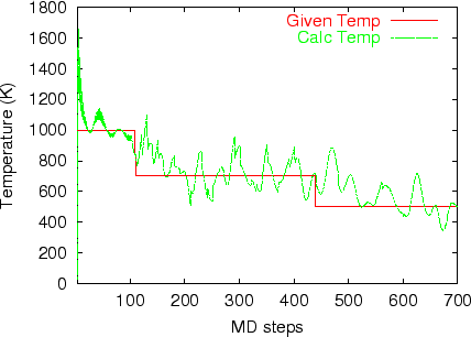
MD steps. The third and fourth columns give a given temperature T_give and a scaling parameter alpha in the interval. In this velocity scaling velocities are scaled by


      where T_given and T_calc are a given and calculted temperatures, respectively. After the final MD step given in the specification 'MD.TempControl', the NVT ensemble is switched to a NVE ensemble. Calculated quantities at every MD step are stored in an output file '*.ene'. Although you can find the details in 'iterout.c', several quantities are summarized for your convenience as follows:
               1:    MD step
               2:    MD time
              14:    kinetic energy of nuclear motion, Ukc (Hartree)  
              15:    DFT total energy, Utot (Hartree)  
              16:    Utot + Ukc (Hartree)  
              17:    Fermi energy (Hartree)  
              18:    Given temperature for nuclear motion (K)        
              19:    Calculated temperature for nuclear motion (K)        
              22:    Nose-Hoover Hamitonian (Hartree)  
            
      which means that the first and second columns correspond to MD step and MD time, and so on. As an example, we show a result for the velocity scaling MD of a glycine molecule (input file) in the following figure.
            
              gnuplot> "gly_VS.ene" u 1:18 w l,"gly_VS.ene" u 1:19 w l


      We see that the temperature in a molecule oscillates around the given temperature. Also for visualization of molecular dynamics an output file '*.md' can be easily animated using free software xmakemol .

    (2) Nose-Hoover molecular dynamics

      Nose-Hoover molecular dynamics (S. Nose, J. Chem. Phys. 81, 511 (1984); S. Nose, Mol. Phys. 52, 255 (1984); G. H. Hoover, Phys. Rev. A 31, 1695 (1985)) is supported to perform NVT ensemble molecular dynamics by the following keyword:
               MD.Type          NVT_NH            # NOMD|Opt|NVE|NVT_VS|NVT_NH
            
      Then, in this NVT molecular dynamics the temperature for nuclear motion can be controlled by
            <MD.TempControl
              4
                1  1000.0
              100  1000.0
              400   700.0
              700   600.0
            MD.TempControl>
            
      The beginning of the description must be <MD.TempControl, and the last of the description must be MD.TempControl>. The first number '4' gives the number of the following lines to control the temperature. In this case you can see that there are four lines. Following the number '4', in the consecutive lines the first and second columns give the number of MD steps and a given temperature for nuclear motion. The temperature between the interval is given by a linear interpolation. Although the same keyword 'MD.TempControl' as used in the velocity scaling MD is utilized in this specification, it is noted that the format is different from each other. 
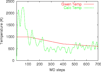
In addition to the specification of 'MD.TempControl', you must specify a mass of heat bath by the following keyword:
              NH.Mass.HeatBath          30.0      # default = 20.0   
            
      In this specification, we use a unit that the weight of a proton is 1.0. Calculated quantities at every MD step are stored in an output file '*.ene' as explained in 'Velocity scaling molecular dynamics'. As an example, we show a result for Nose-Hoover MD of a glycine molecule (input file) in the following figure.
            
              gnuplot> "gly_NH.ene" u 1:18 w l,"gly_NH.ene" u 1:19 w l


      We see that the temperature in a molecule oscillates around the given temperature. Also for visualization of molecular dynamics an output file '*.md' can be easily animated using free software xmakemol .

    (3) NVE molecular dynamics

      The option for NVE molecular dynamics was changed as follows:
               MD.Type          NVE            # NOMD|Opt|NVE|NVT_VS|NVT_NH
            
      It should be noted that the old option 'Constant_Energy_MD' is not available anymore.

    (4) Improvement of calculation of matrix elements for neutral atom potential

      Although a projector expansion scheme of the neutral atom potential has been developed in OpenMX1.5 and OpenMX1.51, we moreover improved the calculation of matrix elements for the neutral atom potential in order to avoid 'eggbox' effect that the total energy oscillates as a function of reaction coordinate. In OpenMX1.6, one- and two-center integrals in matrix elements for the neutral atom potential are accurately calculated in Fourier space, while the projector expansion scheme is employed for only three-center integrals. There is no additional keyword for this development.

    (5) Bugs fixed

      Several bugs in OpenMX Ver. 1.51 were fixed.

    (6) Tips in the installation (Reported by Dr. D. H. Chi at Hanoi Univ.)

      When the latest version (Version 3.0.1) of FFTW is linked to OpenMX, it seems that there are several problems which hamper the installation, although we have never solved this problem. However, the version 2.1.5 of FFTW can be successfully linked to OpenMX. Since only the simplest routine (1D-FFT) in FFTW is employed, we guess that the use of the latest version might not be so effective for decrease of computational time.

6/May/2004

OpenMX1.51 was released.

A revision of OpenMX1.5 is released as OpenMX1.51, since we found a serious problem in OpenMX1.5, which is related to the convergence in the projector expansion of the neutral atom potential.

    (1) Revision of projector expansion of the neutral atom potential

      The neutral atom potential is expanded by the spherical harmonic functions with the angular momentum quantum number up to Lorb+4 in OpenMX1.5, where Lorb is the maximum angular momentum quantum number of basis orbitals. However, if Lorb is greater or equal than 3 (f-orbital), we found that a satisfactory convergence is not achieved. Therefore, the angular momentum quantum number up to Lorb+6 is employed in this projector expansion in OpenMX1.51, which provides a good convergence in almost cases we tested. There is no additional keyword for this revision.

28/Apr./2004

OpenMX1.5 (with user's manual) was released.

The main features of the modifications are as follows (see also the manual):

    (1) Relativistic effects

      Relativistic effects can be incorporated by a fully relativistic and a scalar relativistic pseudo potentials ( A. H. MacDonald and S. H. Vosko, J. Phys. C: Solid State Phys. 12, 2977 (1979); G. B. Bachelet, D. R. Hamann, and M. Schluter, PRB 26, 4199 (1982); G. Theurich and N. A. Hill, Phys. Rev. B 64, 073106 (2001)). To include relativistic effects, you have to generate fully relativistic j-dependent pseudo potentials or scalar relativistic pseudo potentials using ADPACK before the calculations of OpenMX. See also the Section 'Relativistic effects' in the manual for the details.

    (2) Spin-orbit coupling

      If you use a fully relativistic j-dependent pseudo potentials. You can include spin-orbit coupling by the following keyword
              scf.SpinOrbit.Coupling      on         # On|Off, default=off
            
      If you use a fully relativistic j-dependent pseudo potential, and set the keyword 'OFF', then the j-dependent pseudo potential are automatically averaged with a weight of j-degeneracy when it is read by OpenMX, which corresponds to a scalar relativistic pseudo potential. See also the Section 'Relativistic effects' in the manual for the details.

    (3) Non-collinear DFT

      Fully unconstrained non-collinear density functional theories (DFT) are supported including the spin-orbit coupling (SOC) (U. Von. Barth and L. Hedin, J. Phys. C: Solid State Phys. 5, 1629 (1972); J. Kubler, K-H. Hock, J. Sticht, and A. R. Williams, J. Phys. F: Met. Phys. 18, 469 (1988); J. Sticht, K-H. Hock, and J. Kubler, J. Phys.: Condens. Matter 1, 8155 (1989); T. Oda, A. Pasquarello, and R.Car, Phys. Rev. Lett. 80, 3622 (1998)). When the non-collinear DFT is performed, the following option for the keyword 'scf.SpinPolarization' is available.
               scf.SpinPolarization        NC        # On|Off|NC
            
      If the option 'NC' is specified, wave functions are expressed by a two components spinor. An initial spin orientation of each site is given by
            <Atoms.SpeciesAndCoordinates           
              1  Cr    1.07400   1.07400   0.00000    4.0  8.0   90.0  90.0  1  
              2  Cr   -1.07400   1.07400   0.00000    4.0  8.0   90.0 -90.0  1
              3  Cr   -1.07400  -1.07400   0.00000    4.0  8.0   90.0  90.0  1 
              4  Cr    1.07400  -1.07400   0.00000    4.0  8.0   90.0 -90.0  1
              5  Cr    0.00000   0.00000   1.90000    7.0  5.0    0.0   0.0  1
            Atoms.SpeciesAndCoordinates>
            
      The Euler angles, theta and phi, to determine the spin orientation are given by the 8th and 9th columns in the specifination of '<Atoms.SpeciesAndCoordinates'. The final 10th column is a switch for determining whether the spin orientation is relaxed during the SCF calculation. '1' means that the spin orientation is relaxed. '0' means that the spin orientation is fixed at the initial orientation. See also the Section 'Non-collinear DFT' in the manual for the details.

    (4) Charge doping

      Charge doping is supported for both the electron and hole dopings by the following keyword.
              scf.system.charge     1.0     # default=0.0
            
      The plus and minus signs correspond to hole and electron dopings, respectively. A partial charge doping is also possible. The excess charge given by the keyword 'scf.system.charge' is compensated by a uniform background opposite charge, since FFT is used to solve Poisson's equation in OpenMX.

    (5) Decomposed Mulliken analysis

      In addition to the Mulliken charge projected to each atom, a decomposed Mulliken charge to each orbital is also suppoted by default. The result is stored in *.out.

    (6) Voronoi charge analysis

      Voronoi charge of each atom is calculated by integrating electron and spin densities in a Voronoi polyhedron. The Voronoi polyhedron is constructed from smeared surfaces which are defined by a Fuzzy cell partitioning method (A. D. Becke and R. M. Dickson, J. Chem. Phys. 89, 2993 (1988)). If you would calculate Voronoi charge, specify the following keyword in your input file:
             Voronoi.charge      on       # on|off, default = off
            
      The result is stored in *.out.

    (7) Electro-static potential fitting

      The electro-static potential (ESP) fitting method is supported to determine an effective charge of each atom ( U.C.Singh and P.A.Kollman, J.Comp.Chem. 5, 129(1984); L.E.Chirlian and M.M.Francl, J.Com.Chem. 8, 894(1987); B.H.Besler, K.M.Merz Jr. and P.A.Kollman, J.Comp.Chem.11,431(1990) ). See also the Section 'Charge analysis' in the manual for the details.

    (8) Exchange coupling parameter (Provided by M. J. Han and J. Yu at SNU)

      To analyze spin-spin interactions, exchange coupling parameters between two localized spins can be evaluated based on perturbative Green's functions (A. I. Liechtenstein, M. I. Katsnelson, V. P. Antropov, and V. A. Gubanov, J. Mag. Mag. Mat. 67, 65 (1987)). This release is tentative for our collaborators. We are thinking about developing from the current version to more sophisticated theory and code. See also the Section 'Exchange coupling parameter' in the manual for the details.

    (9) Optical conductivity (Provided by H. Kino at NIMS)

      The optical conductivity can be evaluated within linear response theory. This release is tentative for our collaborators. We are thinking about developing from the current version to more sophisticated theory and code. See also the Section 'Optical conductivity' in the manual for the details.

    (10) Analysis of difference in two Gaussian cube files

      A utility tool is provided to generate a Gaussian cube file which stores the difference between two Gaussian cube files for total charge density, spin density, and potentials. If you analyze the difference between two states, the tool would be helpful. See also the Section 'Analysis of difference in two Gaussian cube files' in the manual for the details.

    (11) Analysis of difference in two geometrical structures

      A utility tool is provided to analyze the difference between two geometrical coordinates in two xyz files which store Cartesian coordinates. The following three analyses are supported: a root mean square of deviation (RMSD) between two Cartesian coordinates, a mean deviation (MD) between two Cartesian coordinates, and a mean deviation between bond lengths (MDBL). If you analyze the difference between two structures, the tool would be helpful. See also the Section 'Analysis of difference in two geometrical structures' in the manual for the details.

    (12) Projector expansion of the neutral atom potential

      When the interaction energy of a weak binding system is calculated, we tend to meet an 'eggbox' effect that the total energy oscillates as a function of reaction coordinate, since a finite real space mesh is used for numerical integrations. The 'eggbox' effect mainly comes from the neutral atom potential and partial core correction (PCC) charge, since they are highly localized around atomic cores. To remove the 'eggbox' effect, we have developed a method in which the neutral atom potential is expanded by projector operators. Therefore, the 'eggbox' effect by the neutral atom potential might disappear. However, the 'eggbox' effect by the PCC charge still remains, which means that we have to use a shallow PCC charge to avoid the 'eggbox' effect. If you want to compare the projector expansion and the real space grid integration of the neutral atom potential, then the following keyword is available
             scf.ProExpn.VNA      on       # on|off, default = on
            
      If the keyword is 'on', this means the projector expansion, otherwise the real space grid integration of the neutral atom.

    (13) Bugs fixed

      Several bugs in OpenMX Ver. 0.8 were fixed.

    (14) Manual revised

      The manual of OpenMX was revised.

3/Apr./2004

ADPACK1.5 (with user's manual) was released .

The main features of the modifications are as follows (see also the manual):

    (1) Fully relativistic treatment

      In addition to a scalar relativistic treatment, a fully relativistic treatment was supported (A. H. MacDonald and S. H. Vosko, J. Phys. C: Solid State Phys. 12, 2977 (1979); G. B. Bachelet, D. R. Hamann, and M. Schluter, PRB 26, 4199 (1982)). Therefore, now three options are available for the keyword, eq.type as follows:
             eq.type          dirac    # sch|sdirac|dirac
            
      where 'sch', 'sdirac', and 'dirac' mean the Schrodinger equation (no relativistic effect), a scalar relativistic treatment, and a full relativistic treatment of Dirac equation, respectively. Although eq.type=dirac means the scalar relativistic treatment in ADPACK1.3, the scalar relativistic treatment is specified by 'sdirac' in ADPACK1.5. In the scalar relativistic treatment, the coupled Dirac equations are averaged with a weight of j-degeneracy, and solved by taking account of both the majority and minority components of radial wave function. Thus, the scalar relativistic treatment includes explicitly kinematic relativistic effects (Darwin and mass velocity terms), and implicitly averaged spin-orbit coupling (no energy splitting). On the other hand, in the full relativistic treatment, j-dependent Dirac equations are solved including both the majority and minority components of radial wave function. Thus, energy splitting by spin-orbit coupling is also considered.

    (2) Restart (supported by Dr. Kino)

      For an atom with a large atomic number, all electron calculation requires a considerable computational time. So, it is hard to determine optimal cutoff radii and other parameters in the pseudo potential generation in a trial and error way. Therefore, it is desirable to reduce the computational time that results of the all electron calculation are stored in a file and skip the all electron calculation when we regenerate pseudo potentials in different parameters. To do this, two keywords, System.UseRestartfile and System.Restartfile, are available.
             System.UseRestartfile   YES           # NO|YES, default=NO
            
             System.Restartfile      C0_Rest       # default=null
            
      If the keyword, System.UseRestartfile, is specified as YES, a restart file which contains informations of all electron calculation is used in order to skip all electron calculation. If there is no restart file, a restart file is generated in case of System.UseRestartfile=YES. If System.UseRestartfile=YES, then the name specified by the keyword, System.Restartfile, is refered to as a restart file.

    (3) Bugs fixed

      Several bugs in ADPACK Ver. 1.3 were fixed.

    (4) Manual revised

      The manual of ADPACK was revised.

17/Nov./2003

OpenMX0.8 was released.

The main features of the modifications are as follows:

    (1) GGA (Generalized Gradient Approximation)

      For the exchange-correlation term, GGA (J. P. Perdew, K. Burke, and M. Ernzerhof, Phys. Rev. Lett. 77, 3865 (1996)) becomes now available. The specification for the keyword, 'scf.XcType' is as follows:
             scf.XcType          GGA-PBE 
            
      You can specify either the non-spin or spin polarization calculation based on GGA using the keyword, scf.SpinPolarization.

    (2) Analytic forces

      Fully analytic forces were implemented, which are derived from derivatives of a discretized form of the total energy without any approximation. Therefore, the calculated forces are consistent with the total energy in any quality of cutoff energy for numerical integration and Poisson's equation, which could be highly useful for geometry optimization.

    (3) External electric field

      The SCF calculation and geometry optimization under an uniform external electric field are supported. If you want to apply an electric field of 1.0 GV/m (10^9 V/m) along a-axis, then please specify as follows:
             scf.Electric.Field     1.0  0.0  0.0
            
      The sign of electric field is for electrons. When the uniform external electric field is applied to a periodic system, discontinuities of the potential are introduced. For molecular systems, the discontinuities are located in the vacuum resion. Thus, numerical instabilities may not be induced. On the other hand, you might meet numerical instabilities due to the discontinuities for bulk systems.

    (4) Orbital optimization restricted to species

      A constrained orbital optimization scheme was developed, in which basis orbitals of the same species name, that you define in 'Definition.of.Atomic.Species', are treated as the same orbitals. The specification for the keyword, 'orbitalOpt.Method' as follows:
             orbitalOpt.Method            species
            
      The PAOs for proteins, DNA, and RNA were optimized using the constrained orbital optimization scheme.

    (5) Bugs fixed

      Several bugs in OpenMX Ver. 0.3 were fixed.

18/Oct./2003

OpenMX0.3 (with user's manual) was released.

We rename ABRED as OpenMX (Open source package for Material eXplore), because the code is significantly growing as a more general material simulator.

The main features of the modifications are as follows: (See also the manual of OpenMX as for the details)

    (1) Parallel execution by MPI (message passing interface)

      The program code was fully developed for parallel execution using MPI (message passing interface). Coupling of the parallel execution and the O(N) method enables us to calculate large-scale systems including more than 1000 atoms.

    (2) Divide-conquer O(N) method

      The divide-conquer (DC) method (W.Yang, Phys.Rev.Lett. 66, 1438 (1991)) was employed as a O(N) method in OpenMX, since we found that the DC method is more robust than our O(N) recursion method.

    (3) Interface for developers

      An useful user interface is provided for developers. If you want to make use of Kohn-Sham Hamiltonian, overlap, and density matrices, you only have to include libraries in your codes.

    (4) Constrained relaxation (supported by Dr. Kino)

      It is possible to optimize geometrical structures with a constraint in which atoms can be fixed in the initial position. Then, please specify 'Constraint_Opt' for the keyword, MD.type. For instance, if you want to fix two atoms C(1) and H(2) in the methane molecule, the geometry by <Atoms.SpeciesAndCoordinates is specified as follows:
            <Atoms.SpeciesAndCoordinates
              1   C      0.300000    0.000000    0.000000     2.0  2.0  0
              2   H     -0.889981   -0.629312    0.000000     0.5  0.5  0
              3   H      0.000000    0.629312   -0.889981     0.5  0.5  1
              4   H      0.000000    0.629312    0.889981     0.5  0.5  1
              5   H      0.889981   -0.629312    0.000000     0.5  0.5  1
            Atoms.SpeciesAndCoordinates>
            
      In the final column, 0 means that the atom is fixed at the initial position, and 1 means that the atom is relaxed. If you specify the other keywords for MD.type, then you do not need add the number in the final column.

    (5) Automatic determination of the cell size (supported by Dr. Kino)

      When you calculate an isolated system, you are required to provide a super cell so that the isolated system does not overlap with the image systems in the repeated cells. The larger cell size can cause a numerical inefficiency, since a larger number of grids are used in the solution of the Poisson's equation in this case. Therefore, the use of the minimum cell size is desirable in terms of computational efficiency. OpenMX supports the requirement. If you remove the specification for the cell size, that is, from <Atoms.UnitVectors to Atoms.UnitVectors>, then the minimum cell size is automatically determined. The determined cell vectors are displayed in the standard output.

    (6) Bugs fixed

      Several bugs in ABRED Ver. 1.6 were fixed.

25/June/2003

A database of PAO for proteins was released.

25/June/2003

A database of PAO for proteins was released.

9/June/2003

The manual of B-BOP was released.

9/June/2003

B-BOP1.1 was released.

2/June/2003

The manual of ABRED was revised.

2/June/2003

ABRED (Ver. 1.6) was released.

(A) The main features of the modifications are as follows:

    (1) The dynamic memory allocation
      The dynamic memory allocation was implemented. So, the shell script running by abred.sh was eliminated. This development releases us from a problem of memory allocation and the bother of recompiling. In addition to this, the allocation memory was optimized, so that the minimum memory size is used for your input file.

    (2) Band dispersion
      The calculation of the band dispersion was supported by Dr. Kino. The details are described the revised manual.

    (3) DOS and LDOS
      The calculation of the density of states (DOS) and the local DOS (LDOS) was supported by Dr. Kino. The details are described the revised manual.

    (4) Visualizaion
      Molecular orbitals, electron densities, potentials can be visualized. The details are described the revised manual.

    (5) Orbital optimization
      The output of the orbital optimization was improved. The details are described the revised manual.

    (6) Dipole moment
      The calculation of the dipole moment was supported. The result is outputted in the standard out and *.out.

    (7) Change of the format in Atoms.SpeciesAndCoordinates
      The new format is as follows:
         <Atoms.SpeciesAndCoordinates
           1   C      0.000000    0.000000    0.000000     2.0  2.0 
           2   H     -0.889981   -0.629312    0.000000     0.5  0.5
           3   H      0.000000    0.629312   -0.889981     0.5  0.5
           4   H      0.000000    0.629312    0.889981     0.5  0.5
           5   H      0.889981   -0.629312    0.000000     0.5  0.5
         Atoms.SpeciesAndCoordinates>
           
    Please don't forget to attach a sequential serial number for identifying atoms in the first column.

9/April/2003

ABRED (Ver. 1.3) was released.

The main features of the modifications are as follows:

    (1) The f-orbital was supported.
      Two subroutines, Get_dOrbitals.c and Get_Cnt_dOrbitals.c, were modified.

    (2) The Pulay method were modified.
      Two subroutines, DIIS_Mixing_DM.c and GR_Pulay.c, were modified.
      The modified two routines provide a rapid convergence in the SCF calculations compared to the previus version even for metallic systems. The main idea to accelerate the SCF convergence was to correct the optimized density matrix, rho_opt, by using an optimized residual density matrix, R_opt, as follows:
             rho_inp = rho_opt + alpha*R_opt,
            
      where alpha is a parameter, ranging from 0 to 1, which can vary automatically. When 'scf.Mixing.Type=Rmm-Diis' or 'scf.Mixing.Type=Gr-Pulay' is used, the following recipes are helpful to obtain the convergence of SCF calculations:

        (a) Use a rather larger value for scf.Mixing.StartPulay.
        Before starting the Pulay like mixing, achieve a convergence at some level. An appropriate value may be 10 for scf.Mixing.StartPulay.

        (b) Use a rather larger value for 'scf.ElectronicTemperature' in case of metallic systems.
        When 'scf.ElectronicTemperature' is small, numerical instabilities appear often.

        (c) Look for an appropriate value for 'scf.Mixing.History'.
        In most cases, 'scf.Mixing.History=7' could be a good value.


    (3) LSDA calculations were accelerated.
      Now, 'LDA', 'LSDA-CA', and 'LSDA-PW' are available for the keyword, 'scf.XcType', where 'LSDA-CA' uses the local spin density functional of Ceperley-Alder (D.M.Ceperley and B.J.Alder, Phys.Rev.Lett., 45, 566(1980)), LSDA-PW uses the local spin density functional of Perdew-Wang, in which the gradient of density is set to zero in their GGA formalism (J.P.Perdew and Y.Wang, Phys.Rev.B 45, 13244 (1992)). Note:'LSDA-CA' is faster than 'LSDA-PW'.

    (4) The memory size was analyzed.
      The analysis of the memory size is outputted to a file, *.memory, where * means 'System.Name' your specified. The modification of program to analyze the memory size was done by Dr. Kino at NIMS. Thanks.

9/April/2003

ADPACK (Ver. 1.3) was released.

(A) The main features of the modifications are as follows:

    (1) The scalar relativistic treatment was supported.
      ref., D.D.Koelling and B.N.Harmon, J.Phys.C: Solid State Phys. 10, 3107 (1977)

    (2) The pseudo potentials generation including semicore states was supported.
      ref., P.E.Blochl, PRB 41, 5414 (1990); J.M.Soler et al., J.Phys:Condens.Matter 14, 2745 (2002)

    (3) In additon to KB projector, the Blochl projector was supported.
      ref., P.E.Blochl, PRB 41, 5414 (1990);

    (4) The logarithmic derivatives of wave functions became available.
      ref., G.B.Bachelet, D.R.Hamman, and M.Schluter, PRB 26, 4199 (1982); X.Gonze et al., PRB 41, 12264 (1990)

    (5) The ghost states of pseudo potentials can be detected.
      X.Gonze et al., PRB 41, 12264 (1990); D.M.Bylander and L.Kleinman, PRB 41, 907 (1990)


(B) The eight new keywords are added.

    eq.type
    The keyword, eq.type, specifies the type of equation. For the non-relativistic Kohn-Sham equation, please specify 'sch'. On the other hand, for the scalar relativistic Kohn-Sham equation, please specify 'dirac'.

    Blochl.projector.num
    The keyword, Blochl.projector.num, specifies the number of projectors for each L-component in separable pseudo potentials. If you specify 1 for Blochl.projector.num, this means the Kleinman and Bylander (KB) separable pseudo potentials. As the number of Blochl.projector.num increases, the separable pseudo potential behaves like the semilocal non-separable pseudo potential. We recommend you to use 2 or 3 for Blochl.projector.num in order to increase the transferability of the separable pseudo potential. We guess that you might consider the increase of computational efforts due to the increasing projectors. However, the matrix elements for the non-local part are evaluated outside the SCF loop. Therefore, the computational demands for the larger projectors are quite small. For the details, see the origial paper (P.E.Blochl, PRB 41, 5414 (1990)).

    log.deri.RadF.calc
    In case of 'calc.type=VPS', if you want to calculate the logarithmic derivatives of radial wave functions for the all electron potential, semilocal pseudo potentials, and separable pseudo potentials, then, please specify ON for the keyword, log.deri.RadF.calc. If not so, please specify OFF. The calculated logarithmic derivatives are outputted to the file, *.ld0,*.ld1,..., where * means 'System.Name' your specified, the number attached to the last of the file extention 'ld' is the angular momentum number L. In these files, the first column is energy, the second (D0), third (D1), and fourth (D2) columns are the logarithmic derivatives of radial wave functions for the all electron potential, the semilocal non-separable pseudo potential, and the separable pseudo potential, respectively. In addition to the output of logarithmic derivatives to the files, an useful quantities, I0 and I1, are evaluated in order to discriminate the transferability of the separable pseudo potentials by


    Ideally, the maximum transferability can be obtained when I0 and I1 are zero. So, it is desireable to make pseudo potentials with small I0 and I1 as much as possible. I0 and I1 are outputted on the standard output (your display).

    log.deri.MinE
    In case of 'calc.type=VPS' and 'log.deri.RadF.calc=ON', the keyword, log.deri.MinE, gives the lower bound of energy used in the calculation of logarithmic derivatives of radial wave functions.

    log.deri.MaxE
    In case of 'calc.type=VPS' and 'log.deri.RadF.calc=ON', the keyword, log.deri.MaxE, gives the upper bound of energy used in the calculation of logarithmic derivatives of radial wave functions.

    log.deri.num
    In case of 'calc.type=VPS' and 'log.deri.RadF.calc=ON', the keyword, log.deri.MaxE, gives the number of partitioning for the energy range from 'log.deri.MinE' to 'log.deri.MaxE'.

    log.deri.R
    In case of 'calc.type=VPS' and 'log.deri.RadF.calc=ON', the keyword, log.deri.R, gives the radius at which the logarithmic derivatives of radial wave functions are evaluated. The keyword, log.deri.R, is specifid for each angular momentum number L as follows:
       <log.deri.R
        0  2.0   
        1  2.0
       log.deri.R>
      
    The beginning of the description must be <log.deri.R, and the last of the description must be log.deri.R>. The first column is the angular momentum number L, and the second column is the radius at which the logarithmic derivatives of radial wave functions are evaluated.

    ghost.check
    In case of 'calc.type=VPS', if you want to check whether there are ghost states for the generated separable pseudo potentials, please specify ON for the keyword, ghost.check. If not so, please specify OFF for the keyword. The calculation result appears on the standard output (your display).


(C) Generation of pseudo potentials including semicore states

    The pseudo potentials including semicore states can be evaluated using ADPACK1.3. The following example is for a sodium atom:
     <pseudo.NandL
      0  3  0  1.8
      1  3  1  2.3
      2  4  0  1.8
      3  4  1  2.3 
     pseudo.NandL>
  

(D) A new outputted file, *.loc

    In case of 'calc.type=VPS', the local part, Vlocal, of pseudo potentials is outputted to a file, *.loc, where * means 'System.Name' your specified. The datum are outputted in order of r, log(r), Vlocal.

(E) Important notices

    The format of *.vps, where * means 'System.Name' your specified, is a littel bit changed. Therefore, the generated file, *.vps, can be read in the version 1.3 of ABRED. The version 1.2 of ABRED can NOT read the new format of *.vps. However, ABRED1.3 can read the both old and new formats of *.vps.

13/Feb/2003

The manual of ADPACK was revised.

12/Feb/2002

ADPACK (Ver. 1.1) was released.

K.Lee_and_Han_Report_9/Feb/2003 was fixed.
S.Lee_Report_9/Feb/2003 was fixed.
Kino_Report_11/Feb/2003 was fixed.
Ozaki_Report_12/Feb/2003 was fixed.

The ten parameters are added.

scf.Init.Mixing.Weight
The keyword, scf.Init.Mixing.Weight, gives a mixing weight first used by the simple mixing method and the GR-Pulay method. The valid range is 0< scf.Init.Mixing.Weight <1.

scf.Min.Mixing.Weight
The keyword, scf.Init.Mixing.Weight, gives the lower limit of a mixing weight the simple mixing method.

scf.Max.Mixing.Weight
The keyword, scf.Max.Mixing.Weight, gives the upper limit of a mixing weight the simple mixing method.

local.type
The keyword, local.type, specifies a way for generating the local part of pseudo potentials. "Simple" means that a l-component of pseudo potential, specified by the keyword(local.part.vps), is used as the local part. "Polynomial" means that the local part for the inside of a cutoff radius is generated using a polynomial and that the outer part is proportional to -1/r. At the cutoff radius the two parts are connected so that up to third derivatives are continuous.

local.cutoff
When "Polynomial" is used for the keyword, local.type. Please specify the cutoff radius, rc, (a.u.) for the keyword, local.cutoff.

local.origin.ratio
When "Polynomial" is used for the keyword, local.type. The keyword, local.origin.ratio, specifies the value of the local potential at the origin. It should be noted that VL(0) = local.origin.ratio*VL(rc)

search.LowerE
The keyword, search.LowerE, gives the lower bound for searching the eigenstates of pseudo atomic orbitals.

search.UpperE
The keyword, search.LowerE, gives the upper bound for searching the eigenstates of pseudo atomic orbitals.

num.of.partition
The keyword, num.of.partition, gives the number of energy partitioning, ranging from the search.LowerE to the search.UpperE. First, the eigenstates of pseudo atomic orbitals are roughly explored for the partitioned energy range. Then, the eigenstates is refined in the energy range with a correct number of nodes.

matching.point.ratio
The keyword, matching.point.ratio, gives a matching point to connect two wave functions solved from the origin and the distant. It should be noted that matching grid number is matching.point.ratio * grid.num.

12/Feb/2003

[Ozaki_Report_12/Feb/2003]:
T.Ozaki (AIST) reported that ADPACK (1.0a) fails because of the numerical instabilities when he tried to calculate pseudo atomic orbitals (PAO) of a pseudo gold atom with a high confinement wall (20000 Hartree) using ADPACK (1.0a). So, T.Ozaki (AIST) improved ADPACK (1.0a) to generate these stably by introducing a fixed matching point scheme in the routine, Multiple_PAO.c The problem will be removed in the next release of ADPACK.

11/Feb/2003

[Kino_Report_11/Feb/2003]:
H.Kino (NIMS) reported that an unexpected roughness was observed in the the energy curve when he calculated the total energy curve as a function of the bond length of a aluminum dimer using ABRED (Ver.1.0a). In addition to this, he found that the equilibrium bond lenght of a aluminum dimer strongly depends on the choice of local part of pseudo potentials. We consider that one of the reasons could be related to the shape of the local part. So, T.Ozaki (AIST) improved ADPACK (Ver.1.0a) to make a smooth local part using a polynomial.

9/Feb/2003

[S.Lee_Report_9/Feb/2003]:
S.Lee (SNU) reported that the default value is not set when the keyword is excluded in the input file for ADPACK (Ver. 1.0a) and ABRED (Ver.1.0). H.Kino (NIMS) found that the failure is due to a bug in the Inputtool.c. The bug will be removed in the next release of both ADPACK and ABRED.

9/Feb/2003

[K.Lee_and_Han_Report_9/Feb/2003]:
K.Lee (SNU) and M.Han (SNU) reported that ADPACK (1.0a) fails because of the numerical instabilities when they tried to calculate pseudo potentials (VPS) and pseudo atomic orbitals (PAO) of a gold atom using ADPACK (1.0a). So, T.Ozaki (AIST) improved ADPACK (1.0a) to generate these stably by introducing a variable grid range scheme. The problem will be removed in the next release of ADPACK.

31/Jan/2003

Since several bugs of ABRED (Ver. 1.0) were fixed, ABRED (Ver. 1.0a) was released.

17/Jan/2003

ABRED (Ver. 1.0) was released.

24/Dec/2002

ADPACK (Ver. 1.0) was released.