Next: All electron calculation
Up: User's manual of ADPACK
Previous: Test calculation
Contents
An input file, C.inp, is shown below. This input file has a flexible data
format, in which a parameter is given behind a keyword, the order
of keywords is arbitrary, and a blank and a comment can also be described
freely.
  #
  # File Name
  #

  System.CurrrentDir    ./             # default=./
  System.Name            C0
  Log.print              Off           # ON|OFF

  System.UseRestartfile  yes           # NO|YES, default=NO
  System.Restartfile     C0            # default=null

  #
  # Calculation type
  #

  eq.type               sch            # sch|sdirac|dirac
  calc.type             all            # ALL|VPS|PAO
  xc.type               LDA            # LDA|GGA

  #
  # Atom
  #

  AtomSpecies             6
  max.occupied.N           2
  total.electron         6.0
  valence.electron       4.0
  <occupied.electrons
   1   2.0
   2   2.0  2.0
  occupied.electrons>

  #
  # parameters for solving 1D-differential equations
  #

  grid.xmin             -8.0           # default=-7.0 rmin(a.u.)=exp(grid.xmin)
  grid.xmax              2.8           # default= 2.5 rmax(a.u.)=exp(grid.xmax)
  grid.num               2000          # default=4000
  grid.num.output         500          # default=2000

  #
  # SCF
  #

  scf.maxIter              60          # default=40
  scf.Mixing.Type       simple         # Simple|GR-Pulay
  scf.Init.Mixing.Weight 0.10          # default=0.300
  scf.Min.Mixing.Weight  0.001         # default=0.001
  scf.Max.Mixing.Weight  0.800         # default=0.800
  scf.Mixing.History      7            # default=5
  scf.Mixing.StartPulay   9            # default=6
  scf.criterion         1.0e-10        # default=1.0e-9

  #
  # Pseudopotetial, cutoff (A.U.)
  #

  vps.type               TM            # BHS|TM
  number.vps              2
  <pseudo.NandL
   0  2  0  1.50  0.0
   1  2  1  1.62  0.0
  pseudo.NandL>
  Blochl.projector.num    4            # default=1 which means KB-form
  local.type            polynomial     # Simple|Polynomial
  local.part.vps          1            # default=0
  local.cutoff           1.50          # default=smallest_cutoff_vps
  local.origin.ratio     4.00          # default=3.0
  log.deri.RadF.calc      on           # ON|OFF
  log.deri.MinE          -3.0          # default=-3.0 (Hartree)
  log.deri.MaxE           2.0          # default= 2.0 (Hartree)
  log.deri.num             50          # default=50
  <log.deri.R
   0  2.2
   1  2.4
  log.deri.R>
  ghost.check             off          # ON|OFF

  #
  # Core electron density for partial core correction
  #   pcc.ratio=rho_core/rho_V,
  #   pcc.ratio.origin = rho_core(orgin)/rho_core(ip)
  #

  charge.pcc.calc        on            # ON|OFF
  pcc.ratio              0.25          # default=1.0
  pcc.ratio.origin       5.00          # default=6.0

  #
  # Pseudo atomic orbitals
  #

  maxL.pao                2            # default=2
  num.pao                 5            # default=7
  radial.cutoff.pao      5.0           # default=5.0 (Bohr)
  height.of.wall    20000.0            # default=4000.0 (Hartree)
  rising.edge           0.2            # default=0.5(Bohr),r1=rc-rising.edge
  search.LowerE       -3.000           # default=-3.000 (Hartree)
  search.UpperE       20.000           # default=20.000 (Hartree)
  num.of.partition      300            # default=300
  matching.point.ratio  0.67           # default=0.67
The specification of each keyword is as follows:
Common keywords for calc.type=ALL VPSPAO
System.CurrrentDir
The directory that files are output.
System.Name
The file name of output files.
Log.print
The informations during the calculation are output to the standard
output. Specify Log.print=ON when outputting, or Log.print=OFF when
non-outputting. This keyword is used for developers.
System.UseRestartfile
For an atom with a large atomic number, all electron calculation
requires a considerable computational time. So, it is needed to reduce
the computational time when optimal cutoff radii of pseudopotentials
are determined in a trial and error. If the keyword, System.UseRestartfile,
is specified as YES, a restart file which contains informations of all
electron calculation is used in order to skip the all electron calculation.
If there is no restart file, a restart file is generated in case of
System.UseRestartfile=YES.
System.Restartfile
If System.UseRestartfile=YES, then the name specified by the keyword,
System.Restartfile, is refered to as a restart file.
eq.type
The keyword, eq.type, specifies the type of equation.
For the non-relativistic Kohn-Sham equation, please specify 'sch'.
On the other hand, for the scalar and fully relativistic Kohn-Sham equation,
please specify 'sdirac' and 'dirac', respectively.
calc.type
The keyword specifies a calculation type.
The SCF calculation for all electron calculation (ALL), the generation of
pseudopotentials (VPS), or the generation of pseudo-atomic orbitals (PAO) with
a confinement potential are available. In addition to the three schemes,
ALLFEM (FEMLDA) and FEMHF are available for the all electron LDA and HF calculations
using the finite element method (FEM) [11], respectively.
Due to a technical reason during development, two specifications, ALLFEM and FEMLDA are
equivalent to each other.
xc.type
Approximate method (LDA or GGA) used for an exchange
correlation energy, where LDA is a form parametrized by Perdew and Zunger [1],
and GGA is a form proposed by Perdew, Burke, and Ernzerhof [3]. Also, a LDA functional
proposed by Vosko, Wilk, and Nusair is available by LDA-VWN [2].
AtomSpecies
Give the atomic number.
max.occupied.N
Give the maximum number of the principal
quantum number, n, for occupied electrons.
total.electron
Give the total number of electrons in an atom.
It is also possible to give the number of electrons corresponding
to not only a neutral atom, but also a positive or negative charged
atom. However, note that it becomes difficult to achieve the convergence
in the SCF calculation for a negative atom (there are more electrons than
atomic number), since wave functions tend to be delocalized or unbound spatially.
valence.electron
Give the number of electrons of valence electrons.
occupied.electrons
Give the number of electrons occupied in each orbital.
As seen in C.inp, when 1s, 2s, and 2p orbitals of a carbon atom
are occupied by two electrons in consideration of the spin degeneracy,
respectively, they are specified as follows:
  <occupied.electrons
   1   2.0
   2   2.0  2.0
  occupied.electrons>
The beginning of the description must be  occupied.electrons, and
the last of the description must be occupied.electrons
occupied.electrons, and
the last of the description must be occupied.electrons .
.
grid.xmin
The radial Kohn-Sham equation is solved numerically by a modified
Euler type method from both a radial point  near the origin
and a distant radial point
near the origin
and a distant radial point  (a.u.).
Here, a radial point near the origin is specified
by the keyword, grid.xmin. Note that there
is a relation, (a.u.)=exp(grid.xmin).
In case of the FEM calculation, a different type of grid is used.
See the section, FEM calculation, for the detail.
(a.u.).
Here, a radial point near the origin is specified
by the keyword, grid.xmin. Note that there
is a relation, (a.u.)=exp(grid.xmin).
In case of the FEM calculation, a different type of grid is used.
See the section, FEM calculation, for the detail.
grid.xmax
The keyword, grid.xmax, specifies a distant radial point (a.u.)
which begins to solve a Kohn-Sham equation. As well as grid.xmin,
note that (a.u.)=exp(grid.xmax).
The selection of a suitable grid.xmax is dependent on an atom.
For an atom with only localized electrons such as carbon and oxygen,
the use of about 2.5 (a.u.) is recommended as grid.xmax. In case of an atom
such as Na, Ti, Fe with delocalized electrons, the use of about 3.0 (a.u.) or
more is recommended as grid.xmax. Moreover, a large value for grid.xmax should
be used when a atom is charged negatively.
In case of the FEM calculation, a different type of grid is used.
See the section, FEM calculation, for the detail.
grid.num
The radial coordinate  is discretized to solve the radial Kohn-Sham
equation by a modified Euler type method. The number of division is specified
by grid.num. The actual mesh division is done for x (=log(r)) as
dx=(grid.xmax-grid.xmin)/(grid.num-1) rather than for r to cope with large
variations near the origin of potential and wave functions.
In case of the FEM calculation, a different type of grid is used.
See the section, FEM calculation, for the detail.
is discretized to solve the radial Kohn-Sham
equation by a modified Euler type method. The number of division is specified
by grid.num. The actual mesh division is done for x (=log(r)) as
dx=(grid.xmax-grid.xmin)/(grid.num-1) rather than for r to cope with large
variations near the origin of potential and wave functions.
In case of the FEM calculation, a different type of grid is used.
See the section, FEM calculation, for the detail.
grid.num.output
It is possible to change the number of grids for in output files
by the keyword, grid.num.output, although the actual calculation is
performed using grid.num.
scf.maxIter
The maximum number of SCF iterations is specified by the keyword,
scf.maxIter. The SCF loop is terminated at the number specified
by scf.maxIter even if the convergence criterion is not satisfied.
scf.Mixing.Type
A mixing method of generateing an input electron
density at the next SCF step is specified by keyword, scf.Mixing.Type.
Three schemes are available: Simple, GR-Pulay, and Pulay, which are the simple
mixing method, GR-Pulay method (Guaranteed-Reduction Pulay method) [12], and the
Pulay method [13], respectively. The simple mixing method used here
is modified to accelerate the convergence by referring to a convergence history.
So, the use of the simple mixing method is recommended because of its robustness.
scf.Init.Mixing.Weight
The keyword, scf.Mixing.Weight, gives an inital mixing weight
used by all the mixing methods in ADPACK .
The valid range is  scf.Mixing.Weight
 .
.
scf.Min.Mixing.Weight
The keyword, scf.Init.Mixing.Weight, gives the lower limit of
a mixing weight in the simple mixing method.
scf.Max.Mixing.Weight
The keyword, scf.Max.Mixing.Weight, gives the upper limit of a mixing
weight in the simple mixing method.
scf.Mixing.History
In the GR-Pulay and Pulay methods, the input electron density at the next SCF step is
calculated by making use of the output electron densities in the several previous SCF
steps. The keyword, scf.Mixing.History, specifies the number of previous
SCF steps which are taken into account for the calculation. For example,
scf.Mixing.History is specified to be 3, and the SCF step is 6th.
Then, the output electron density at 5, 4, and 3 SCF steps are
taken into account to construct an optimimun input electron density.
scf.Mixing.StartPulay
The SCF step which starts the GR-Pulay or Pulay method is specified by the keyword,
scf.Mixing.StartPulay. The simple mixing method is employed in SCF
steps before starting GR-Pulay or Pulay method.
scf.criterion
The keyword, scf.criterion, specifies a convergence criterion for the
SCF calculation. The SCF iteration is terminated when a condition,
NormRDscf.criterion, is satisfied, where a norm of the deviation
between the input and output electron densities, NormRD, is defined
by
 .
.
Specific keywords fo calc.type=VPSPAO
vps.type
When VPS is chosen for the keyword, calc.type, the keyword, vps.type,
specifies a generation method of pseudopotentials.
Either BHS [5], TM [4], or MBK [6] is available.
number.vps
Give the total number of pseudopotentials that you want to generate.
pseudo.NandL
The keyword, pseudo.NandL, specifies a set of a principal quantum number, N,
and an angular momentum quantum number, L, of pseudopotentials
corresponding to the number of potentials specified by the keyword,
number.vps. For example, if number.vps is chosen to be 2 for
a carbon atom, and the pseudopotentials for 2s and 2p orbitals are
generated, then specify in the following way:
  <pseudo.NandL
   0  2  0  1.3  0.0
   1  2  1  1.3  0.0
  pseudo.NandL>
The first column specifies a serial number beginning from zero,
which is used in the specification of the keyword, local.part.vps.
In the second or third columns, a principal number and an angular
momentum quantum number are given. The fourth column provides
a cutoff radius (a.u.) for the generation of pseudopotentials.
Although an optimum cutoff radius is determined so that the generated
pseudopotential has a smooth shape without distinct kinks and
a lot of nodes, however, the choice is made in a somewhat empirical way.
The fifth column provides an energy at which each pseudopotential is genenerated.
However, if the state is occupied (non-zero occupation), then the eigenenergy is
used instead of the value given by the fifth column. The energy given by the
fifth column is used for only a state with zero occupation. Regardless of the
occupation number, the fifth column has to be provided.
The beginning of the description must be pseudo.NandL, and
the last of the description must be pseudo.NandL.
Blochl.projector.num
The keyword, Blochl.projector.num, specifies the number of
projectors for each L-component in separable pseudopotentials.
If you specify 1 for Blochl.projector.num, this means the Kleinman
and Bylander (KB) separable pseudopotential. As the number of
Blochl.projector.num increases, the separable pseudopotential
converges the semilocal non-separable pseudopotential.
We recommend you to use 2 or 3 for Blochl.projector.num in order to
increase the transferability of the separable pseudopotential.
We guess that you might consider the increase of computational
efforts due to the increasing projectors. However, the matrix
elements for the non-local part are evaluated outside the SCF loop.
Therefore, the computational demand for a larger number of projectors
is quite small.
local.type
The keyword, local.type, specifies a way for generating the local
part of pseudopotentials. 'Simple' means that a l-component of
pseudopotential, specified by the keyword (local.part.vps), is used
as the local part. 'Polynomial' means that the local part for the
inside of a cutoff radius is generated using a polynomial and that
the outer part is proportional to -1/r. At the cutoff radius
the two parts are connected so that up to third derivatives
are continuous.
local.part.vps
When 'Simple' for the keyword, local.type, is used,
the keyword, local.part.vps, specifies the local potential used in the
generation of factorized pseudopotentials. In this specification,
please choose the number of the first column in the specification
of the keyword, pseudo.NandL.
local.cutoff
When 'Polynomial' is used for the keyword, local.type, the cutoff radius,
 (a.u.), at which a polynomial local part is connected to
  ,
is specified by the keyword, local.cutoff, where
,
is specified by the keyword, local.cutoff, where  is the number of valence electrons
in the pseudopotential generation.
is the number of valence electrons
in the pseudopotential generation.
local.origin.ratio
When 'Polynomial' is used for the keyword, local.type.
The keyword, local.origin.ratio, specifies the value of the local potential
at the origin. It should be noted to be
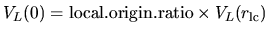 .
.
log.deri.RadF.calc
In case of 'calc.type=VPS', if you want to calculate the
logarithmic derivatives of radial wave functions for the
all electron potential, semilocal pseudopotentials, and
separable pseudopotentials, then, please specify ON for
the keyword, log.deri.RadF.calc. If not so, please specify OFF.
The calculated logarithmic derivatives are output
to the file, *.ld0,*.ld1,..., where * means 'System.Name'
you specified, the number attached to the last of the file
extention 'ld' is the angular momentum number L. In these files,
the first column is energy, the second ( ), third (
 ),
and fourth (
),
and fourth ( ) columns are the logarithmic derivatives of
radial wave functions for the all electron potential, the
semilocal non-separable pseudopotential, and the separable
pseudopotential, respectively. In addition to the output of
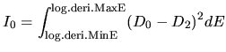
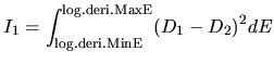
logarithmic derivatives to the files, an useful quantities,
) columns are the logarithmic derivatives of
radial wave functions for the all electron potential, the
semilocal non-separable pseudopotential, and the separable
pseudopotential, respectively. In addition to the output of
logarithmic derivatives to the files, an useful quantities,
 and
and  , are evaluated in order to discriminate the
transferability of the separable pseudopotentials by
, are evaluated in order to discriminate the
transferability of the separable pseudopotentials by
Ideally, the maximum transferability can be obtained when
and are zero. So, it is desireable to make pseudopotentials
with small and . and
are output on the standard output (your display).
log.deri.MinE
In case of 'calc.type=VPS' and 'log.deri.RadF.calc=ON', the keyword,
log.deri.MinE, gives the lower bound of energy (Hartree) used in the
calculation of logarithmic derivatives of radial wave functions.
log.deri.MaxE
In case of 'calc.type=VPS' and 'log.deri.RadF.calc=ON', the keyword,
log.deri.MaxE, gives the upper bound of energy (Hartree) used in the calculation
of logarithmic derivatives of radial wave functions.
log.deri.R
In case of 'calc.type=VPS' and 'log.deri.RadF.calc=ON', the keyword,
log.deri.R, gives the radius (a.u.) at which the logarithmic derivatives
of radial wave functions are evaluated.
If eq.type=sch or eq.type=sdirac, the keyword, log.deri.R,
is specifid for each angular momentum number L as follows:
   <log.deri.R
    0  2.2
    1  2.4
   log.deri.R>
The beginning of the description must be log.deri.R, and the last
of the description must be log.deri.R. The first column is the
angular momentum number L, and the second column is the radius
at which the logarithmic derivatives of radial wave functions
are evaluated.
If eq.type=dirac, the third column is needed as follows:
   <log.deri.R
    0  2.0 1.9
    1  2.0 2.1
   log.deri.R>
where the second and third column give the radii
at which the logarithmic derivatives of radial wave functions
of  and
and  are evaluated, respectively.
ghost.check
In case of 'calc.type=VPS', if you want to check whether there
are ghost states for the generated separable pseudopotentials,
please specify ON for the keyword, ghost.check.
If not so, please specify OFF for the keyword. The calculation
result appears on the standard output (your display).
charge.pcc.calc
A charge density used for a partial core correction (PCC)
to the exchange-correlation functional [14] is calculated by turning
charge.pcc.calc on.
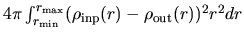
pcc.ratio
The keyword, pcc.ratio, is a parameter in the calculation of
a partial core electron density.
The core electron density is approximated using a fourth order polynomial
below the cutoff radius  at which the ratio
 between the core electron density
  and the valence electron
density
and the valence electron
density  becomes pcc.ratio.
pcc.ratio.origin
The keyword, pcc.ratio.origin, is a parameter in the calculation of
a partial core electron density.
The core electron density is approximated using a fourth order polynomial,
so that the core electron at the origin satisfies a relation,
 =pcc.ratio.origin
 .
.
Specific keywords for calc.type=PAO
maxL.pao
The pseudo-atomic orbitals are generated up to an angular momentum
quantum number, maxL.pao.
num.pao
The number of pseudo-atomic orbitals generated with the same angular
momentum quantum number.
radial.cutoff.pao
The keyword, radial.cutoff.pao, specifies a cutoff radius  (a.u.)
for the pseudo-atomic orbitals.
(a.u.)
for the pseudo-atomic orbitals.
height.of.wall
The keyword, height.of.wall, specifies a height (Hartree) of confinement
wall.
rising.edge
The keyword, rising.edge, controls a shape of rising edge of
the confinement wall. Note that there is a relation
 =
= rising.edge. See also the section, Generation
of pseudo-atomic orbitals.
rising.edge. See also the section, Generation
of pseudo-atomic orbitals.
search.LowerE
The keyword, search.LowerE, gives the lower bound of energy for searching
eigenenergies of pseudo-atomic orbitals.
search.UpperE
The keyword, search.UpperE, gives the upper bound of energy for searching
eigenenergies of pseudo-atomic orbitals.
num.of.partition
The keyword, num.of.partition, gives the number of energy partitioning,
ranging from the search.LowerE to the search.UpperE.
First, the eigenstates of pseudo-atomic orbitals are roughly explored
for the energy ranges partitioned by the keyword, num.of.partition.
Then, the eigenstates are refined in the energy range with a correct
number of nodes.
matching.point.ratio
The keyword, matching.point.ratio, gives a matching point to connect
two wave functions solved from the origin and the distant.
It should be noted that
the matching grid number is given by matching.point.ratio  grid.num.
Next: All electron calculation
Up: User's manual of ADPACK
Previous: Test calculation
Contents
2011-09-28