General

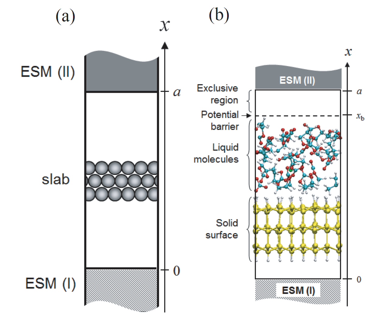
The effective screening medium (ESM) method is a first-principles computational method for charged or biased systems consisting of a slab [86,87,88,89]. In this method, a 2-dimensional periodic and 1-dimensional optional boundary conditions are imposed on a model cell (Fig. 44(a)), and the Poisson's equation is solved under those set of boundary conditions by using the Green's function method. An isolated slab, charged slab, and a slab under an uniform electric field can be treated by introducing the following combinations of semi-infinite media (ESMs).

(a) Isolated slab: vacuum (relative permittivity $\varepsilon=1$) + vacuum

(b) Charged slab: vacuum + ideal metal (relative permittivity $\varepsilon=\infty$)

(c) Slab under an electric filed: ideal metal + ideal metal

Here 'slab' means a system consisting of molecules spaced out 2-dimensionally as well as a slab generally used as a surface model. An isolated slab model can be used for investigations of a polarized substrate, and charged slab model is applicable to a simulation of an electrode surface. A slab model under an electric filed sandwiched between two ideal-metal media would be appropriate for a material located in a metal capacitor. In OpenMX, a unit cell used in an ESM-method calculation is constructed as follows (see Fig. 44(a)):

1. The a-axis of the cell is perpendicular to the b-c plane and is parallel to the x-axis.
2. Two periodic boundary conditions are set in y- and z-axis directions
3. ESMs are placed at the cell-boundaries (x = 0 and a).
4. The origin of the x-axis is set at the cell boundary.
5. A fractional coordinate for x-axis is designated between 0 and 1.

Figure 44: (a) Schematic view of a slab with semi-infinite media (ESMs). ESM (I) and (II) are placed at cell-boundaries, x = 0 and a (a: the length of the cell along x-axis), respectively. (b) An example of a unit cell for a MD calculation of solid surface-liquid interface model system with the ESM method. The slab and ESMs are placed parallel to the y-z plane.

A calculation based on an ESM-method can be performed by the following keyword:

  ESM.switch             on3      # off, on1=v|v|v, on2=m|v|m, on3=v|v|m, on4=on2+EF
  ESM.buffer.range       4.5      # default=10.0 (ang),

where on1, on2, on3, and on4 represent combinations of ESMs, 'vacuum + vacuum', 'ideal metal + ideal metal', 'vacuum + ideal metal', and 'ideal metal + ideal metal under an electric field', respectively. The keyword 'ESM.buffer.range' indicates the width of a exclusive region for atoms with ESM (unit is Å), which is necessary in order to prevent overlaps between wave functions and ESM.

1. ESM.switch = on1:

   Both ESM (I) and (II) are semi-infinite vacuum media. In this case, note that the total charge of a calculation system should be neutral. The keyword 'scf.system.charge' should be set to be zero.

2. ESM.switch = on2:

   Both ESM (I) and (II) are semi-infinite ideal-metal media. One can deal with charged systems. The keyword 'scf.system.charge' can be set to be a finite value.

3. ESM.switch = on3:

   ESM (I) and (II) are a semi-infinite vacuum and ideal metal medium, respectively. One can deal with charged systems. The keyword 'scf.system.charge' can be set to be a finite value.

4. ESM.switch = on4:

   An electric field is imposed on the system with the same combination of ESMs to 'on2'. By using the following keyword, one can impose a uniform electric field on a calculation system;

     ESM.potential.diff        1.0      # default=0.0 (eV),
   

   where one inputs a potential difference between two semi-infinite ideal-metal media with reference to the bottom ideal metal (unit is eV). The electric filed is decided by the length of the cell, a, and the potential difference.

5. In case of MD calculations with the ESM method:

   One can implement MD calculations of solid surface-liquid interface systems with any combinations of ESMs. A surface-model slab and a liquid region should be located as shown in Fig. 44(b). In order to restrict liquid molecules within a given region, an cubic barrier potential can be introduced by using the following keyword (see Fig. 44(b)):

     ESM.wall.position        6.0      # default=10.0 (ang)
     ESM.wall.height        100.0      # default=100.0 (eV),
   

   where 'ESM.wall.position' denotes the distance between the upper edge of the cell and the origin of the barrier potential, $a-x_b$, and 'ESM.wall.height' is the height of the potential (value of potential energy) at $x=x_b+1.0$ (Å). It is also recommended to fix positions of atoms on the bottom of a surface-model slab during a MD run.

Figure 45: Al-Si(111) slab model with vacuum and ideal-metal ESMs; (a) Distributions of excess charge in Al-Si(111) slab, $\rho_{\rm ex}$; (b) Bias-induced changes of Hartree potentials of Al-Si(111) slab, $\Delta V_{\rm H}$. The number of doped charge is -0.01, -0.005, +0.005, and +0.01 e. Each plot is obtained as a difference in difference charge or difference Hartree potential with reference to a neutral slab with the same ESMs.