NVT molecular dynamics by a velocity scaling

A velocity scaling scheme [19] is supported to perform NVT ensemble molecular dynamics simulation by the following keyword:

    MD.Type          NVT_VS    # NOMD|Opt|NVE|NVT_VS|NVT_VS2|NVT_NH

Then, in this NVT molecular dynamics the temperature for nuclear motion can be controlled by

    <MD.TempControl
      3
      100   2  1000.0  0.0  
      400  10   700.0  0.4  
      700  40   500.0  0.7  
    MD.TempControl>

The beginning of the description must be '$<$MD.TempControl', and the last of the description must be 'MD.TempControl$>$'. The first number '3' gives the number of the following lines to control the temperature. In this case you can see that there are three lines. Following the number '3', in the consecutive lines the first column means MD steps and the second column gives interval of MD steps that the velocity scaling is made. For the above example, a velocity scaling is performed at every two MD steps until 100 MD steps, at every 10 MD steps from 100 to 400 MD steps, and at every 40 MD steps from 400 to 700 MD steps. The third and fourth columns give a given temperature $T_{\rm give}$ (K) and a scaling parameter $\alpha$ in the interval, while the temperature in the interval is given by a linear interpolation. In this velocity scaling, velocity is scaled by

$$s = \sqrt\frac{T_{\rm given}+(T_{\rm calc}-T_{\rm given})*\alpha} {T_{\rm calc}}$$

$${\bf v}_{i}' = {\bf v}_{i}\times s$$

where $T_{\rm given}$ and $T_{\rm calc}$ are a given and calculated temperatures, respectively. In 'NVT_VS' the temperature is calculated by using velocities of all the atoms. On the other hand, the local temperature is estimated by the velocity of each atom in 'NVT_VS2', and the velocity scaling is performed by the local temperature. After the final MD step given in the specification 'MD.TempControl', the NVT ensemble is switched to a NVE ensemble. Calculated quantities at every MD step are stored in an output file 'System.Name.ene', where 'System.Name' means 'System.Name'. Although you can find the details in 'iterout.c', several quantities are summarized for your convenience as follows:

         1:    MD step
         2:    MD time
        14:    kinetic energy of nuclear motion, Ukc (Hartree)  
        15:    DFT total energy, Utot (Hartree)  
        16:    Utot + Ukc (Hartree)  
        17:    Fermi energy (Hartree)  
        18:    Given temperature for nuclear motion (K)        
        19:    Calculated temperature for nuclear motion (K)        
        22:    Nose-Hoover Hamiltonian (Hartree)

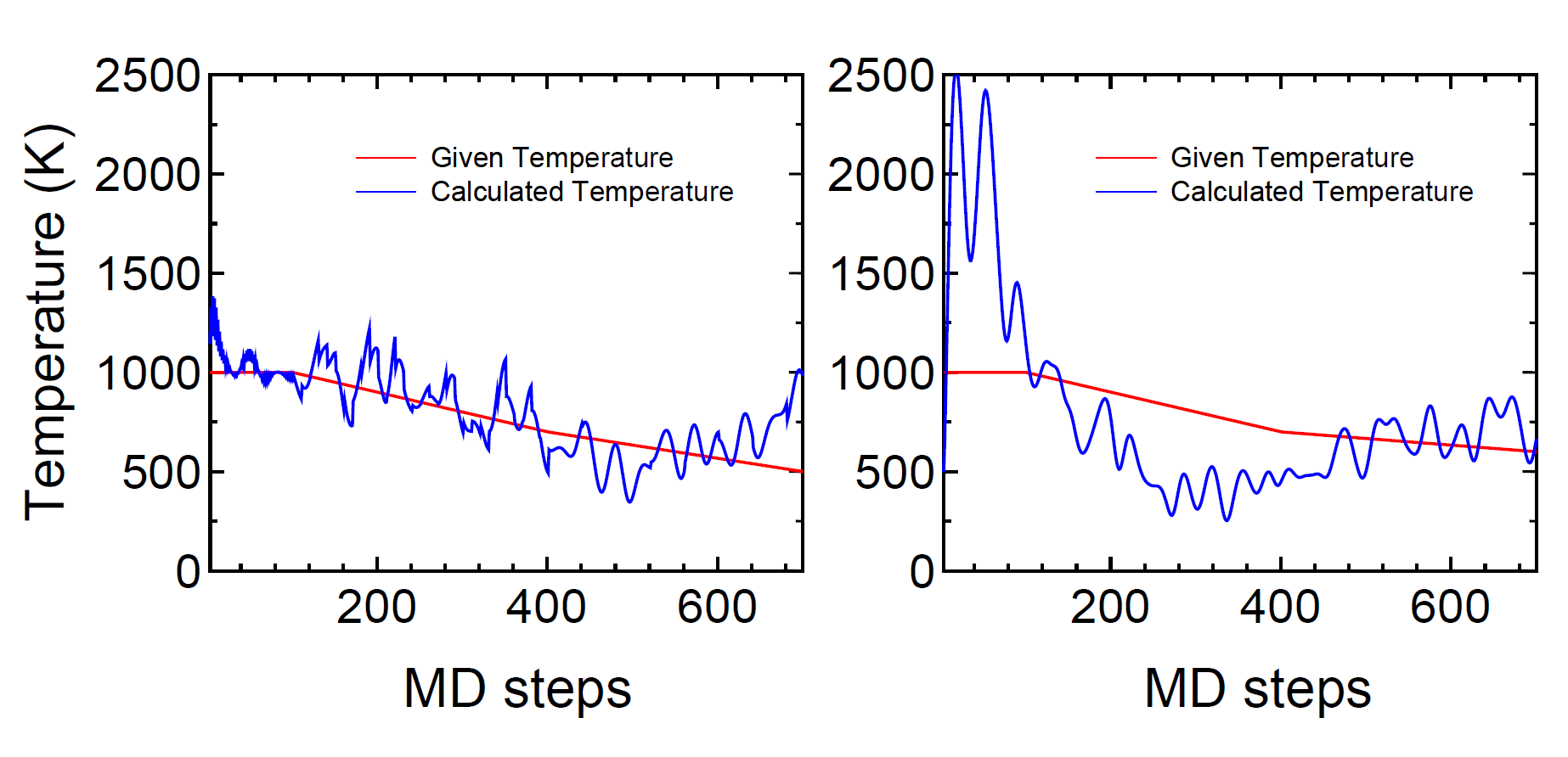
which means that the first and second columns correspond to MD step and MD time, and so on. As an example, we show a result for the velocity scaling MD of a glycine molecule in Fig. 12 (a).

Figure 12: (a) Given and calculated temperatures of a glycine molecule as a function of MD steps in a velocity scaling NVT molecular dynamics. (b) Given and calculated temperatures of a glycine molecule as a function of MD steps in the Nose-Hoover NVT molecular dynamics. The input files are 'Gly_VS.dat' and 'Gly_NH.dat' in the directory 'work', respectively.

We see that the temperature in a molecule oscillates around the given temperature. Also for visualization of molecular dynamics, an output file 'System.Name.md' can be easily animated using free software xmakemol [104] and XCrySDen [66].