General

The 'jx', a post-processing code for OpenMX, provides a way to calculate exchange coupling parameters $J_{ij}$ between two localized spins based on Green's function representation of Liechtenstein formula [17]. In the standard distribution of OpenMX Ver. 3.9, the evaluation is supported for only the collinear calculations of cluster and bulk systems. To acknowledge in any publications by using the functionality, the citation of the references [18,19] would be appreciated.

The program provides three ways to calculate $J_{ij}$ as explained below.

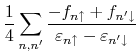
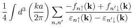
For cluster systems, the program computes exchange coupling constants $J_{ij}$ between atomic sites $i$ and $j$ from the following formula:

$$J_{ij} = \frac{1}{4} \sum_{n,n'} \frac{-f_{n\uparrow}+f_{n'\downarrow}}{\varepsilon_{n\uparrow}-\varepsilon_{n'\downarrow}}$$

$$\times \sum_{\mu,\nu\in i}\sum_{\mu',\nu' \in j} C_{j\mu',n\upa... ...nu\mu} C_{i\mu,n'\downarrow}C^{*}_{j\nu',n'\downarrow} [\hat{P}_{j}]_{\nu'\mu'}$$ (3)

$$\hat{P}_{i} \equiv \hat{H}_{i\uparrow} -\hat{H}_{i\downarrow},$$ (4)

where $\varepsilon_{n\sigma}$ and $\mathbf{C}_{n\sigma}$ represent the corresponding eigenvalue and eigenvector, respectively, indexed by $n$ and $\sigma$ for the Kohn-Sham equation at the wave number $\mathbf{k}$; and $[\hat{P}_{i}]_{\nu\mu}$ and $[\hat{P}_{j}]_{\nu'\mu'}$ represent the partial matrices of the potential difference operator at the sites $i$ and $j$, respectively.

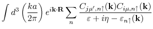
For bulk systems, the program computes exchange coupling constants $J_{i\mathbf{0},j\mathbf{R}}$ between individual sites $i$ and $j$ located at cells $\mathbf{0}$ and $\mathbf{R}$, respectively, from the following formula:

$$J_{i\mathbf{0},j\mathbf{R}} = \frac{1}{2} \sum_{p=1}^{N_{\mathrm{P}}}\tilde{R}_{p}\sum_{\mu,\nu... ...j}]_{\nu'\mu'} G^{+}_{j\mu',i\nu}(\uparrow,\tilde{z}_{p},-\mathbf{R}) \right\}.$$ (5)

where $\tilde{z}_{p}$ and $\tilde{R}_{p}$ are the positive poles and corresponding residues of approximated Fermi functions, $i$ and $j$ are atom indices in a unit cell, $\mathbf{R}$ is a cell index of the second atom, The Green's functions $G^{+}_{j\mu',i\nu}(\uparrow,\varepsilon,-\mathbf{R})$ and $G^{+}_{i\mu,j\nu'}(\downarrow,\varepsilon,\mathbf{R})$ are defined as the following equations:

$$G^{+}_{j\mu',i\nu}(\uparrow,\varepsilon,-\mathbf{R}) \equiv \int d^3\left(\frac{ka}{2\pi}\right)e^{i\mathbf{k}\cdot\mathbf{R}... ...n\uparrow}(\mathbf{k})} {\varepsilon+i\eta-\varepsilon_{n\uparrow}(\mathbf{k})}$$ (6)

$$G^{+}_{i\mu,j\nu'}(\downarrow,\varepsilon,\mathbf{R}) \equiv \int d^3\left(\frac{ka}{2\pi}\right)e^{-i\mathbf{k}\cdot\mathbf{R... ...arrow}(\mathbf{k})} {\varepsilon+i\eta-\varepsilon_{n'\downarrow}(\mathbf{k})}.$$ (7)

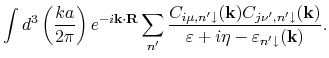
Alternatively, it is also possible to compute the summation of exchange coupling $J_{ij}$ over $\mathbf{R}$ by the following formula:

$$J_{ij} = \sum_{\mathbf{R}}J_{i\mathbf{0},j\mathbf{R}}$$

$$= \frac{1}{4}\int d^3\left(\frac{ka}{2\pi}\right) \sum_{n,n'} \frac... ...})}{\varepsilon_{n\uparrow}(\mathbf{k})-\varepsilon_{n'\downarrow}(\mathbf{k})}$$

$$\times \sum_{\mu,\nu\in i}\sum_{\mu',\nu' \in j} C_{j\mu',n\upa... ...ow}(\mathbf{k})C^{*}_{j\nu',n'\downarrow}(\mathbf{k}) [\hat{P}_{j}]_{\nu'\mu'}.$$ (8)

For the details of Eqs. (3), (5), and (8), see Ref. [18,19].

Figure 37: Schematic of exchange coupling constant between individual sites and that between periodic images.

For users, it might be helpful to explain the difference between Eqs. (5) and (8) by schematics shown in Fig. 37. Figure 37 (a) shows a schematic of interaction between individual sites, which corresponds to Eq. (5). Figure 37 (b) shows a schematic of interaction between periodic images, which corresponds to Eq. (8). When executing, this option can be specified by Flag.PeriodicSum, as explained in the latter subsection.