Numerical atomic basis orbitals from H to Kr: Ver. 1.0

The original has been published in Phys. Rev. B 69, 195113 (2004)

Taisuke Ozaki (JAIST) and Hiori Kino (NIMS)

Abstract:

We present the first systematic study for numerical atomic basis orbitals ranging from H to Kr, which could be used in large scale O($N$) electronic structure calculations based on density functional theories (DFT). The comprehensive investigation of convergence properties with respect to our primitive basis orbitals provides a practical guideline in an optimum choice of basis sets for each element, which well balances the computational efficiency and accuracy. Moreover, starting from the primitive basis orbitals, a simple and practical method for variationally optimizing basis orbitals is presented based on the force theorem, which enables us to maximize both the computational efficiency and accuracy. The optimized orbitals well reproduce convergent results calculated by a larger number of primitive orbitals. As illustrations of the orbital optimization, we demonstrate two examples: the geometry optimization coupled with the orbital optimization of a C$_{60}$ molecule and the pre-orbital optimization for a specific group such as proteins. They clearly show that the optimized orbitals significantly reduce the computational efforts, while keeping a high degree of accuracy, thus indicating that the optimized orbitals are quite suitable for large scale DFT calculations.

I. INTRODUCTION

Atomic orbitals as a basis set have been used for a long time in the electronic structure calculations of molecules and bulks. Especially, in covalent molecular systems, one-particle wave functions are well described by a linear combination of atomic orbitals (LCAO) because of the nature of localization in the electronic states, which is a reason why chemists prefer to use the atomic orbitals, e.g. Gaussian orbitals.[1,2,3,4] On the other hand, in the solid state physics, LCAO has been regarded as a somewhat empirical method such as a tool for an interpolation of electronic structure calculations with a high degree of accuracy.[5] However, during the last decade, LCAO has been attracting much interest from different points of views, since great efforts have been made not only for developing O($N$) methods of the eigenvalue problem,[6,7,8,9,10,11] but also for making efficient and accurate localized orbitals[12,13,14,15,16] as a basis set being suitable for O($N$) methods to extend the applicability of density functional theories (DFT) to realistic large systems. Most O($N$) methods are formulated under an assumption that a basis set are localized in the real space.[11] Therefore, the locality of the atomic orbitals can be fully utilized in DFT calculations coupled with O($N$) methods. In addition, even if a minimal basis set of atomic orbitals is employed for valence electrons, it has been reported that a considerable accuracy is achieved in many systems.[12,17,18,19,20,21] This fact suggests that the matrix size of the eigenvalue problem is notably reduced compared to other localized basis methods such as finite elements method.[22,23] These aspects of LCAO encourage us to employ the atomic orbitals in the large scale O($N$) DFT calculations.

However, several important problems still remain in the applications of LCAO to DFT calculations in spite of these advantages. The most serious drawback in LCAO is the lack of a systematic improvement of atomic orbitals in terms of the computational accuracy and efficiency. One expects that a basis set such as double valence orbitals with polarization orbitals for valence electrons provides a way for balancing a relatively small computational effort and a considerable degree of accuracy. Nevertheless, when a higher degree of accuracy is required, we find the lack of a systematic and simple way for increasing the number of atomic orbitals and for improving the shape of atomic orbitals at a satisfactory level within our knowledge of the LCAO method. Therefore, to overcome the drawback and to benefit the advantages, desirable atomic orbitals as a basis set must be developed with the following features: (i) the computational accuracy and efficiency can be easily controlled by simple parameters as few as possible, (ii) once the number of basis orbitals are fixed, which means that an upper limit is imposed on the computational efforts, the accuracy can be maximized by optimizing the shape of the atomic orbitals. Along this line, recently, accurate basis sets have been constructed in several ways.[12,13,14,15] Kenny et al. constructed a basis set so that atomic orbitals can span the subspace defined by selected and occupied states of reference systems as much as possible.[12] Junquera et al. optimized the shape and cutoff radii of atomic orbitals for reference systems by using the downhill simplex method.[13] However, in these approaches, the serious problem in LCAO has not been solved at a satisfactory level, since the transferability of these optimized orbitals may be restricted to systems similar to the reference systems used for the optimization in terms of atomic environments and states such as the coordination number and the charge state. A more complete treatment for the optimization scheme is to variationally optimize atomic orbitals of each atom located on different environments in a given system.[15,16] Furthermore, it is difficult to control the computational accuracy by simple parameters since the procedure for generating more multiple orbitals than a minimal basis set is not unique in these approaches proposed previously.[12,13]

In this paper, we present the first systematic study of convergence properties for numerical atomic orbitals ranging from H to Kr, in which it is shown that the computational accuracy can be controlled by two simple parameters: a cutoff radius and the number of atomic orbitals. Our comprehensive study not only provides a solution for the above first criterion, but also reveals the limitation in the applicability of LCAO to metallic systems, especially, alkaline and alkaline earth metals. Moreover, starting from our primitive orbitals, a simple and practical method is presented for variationally optimizing numerical atomic orbitals of each atom in a given system based on the force theorem. The orbital optimization scheme enables us to maximize the computational accuracy within a given number of basis orbitals, which fulfills the above second criterion. This paper is organized as follows. In Secs. II and III, we present a method for generating numerical atomic orbitals, and show the convergence properties within DFT in dimers ranging from H to Kr and selected bulks with respect to a cutoff radius and the number of orbitals. In Sec. IV, a simple method is presented for variationally optimizing numerical atomic orbitals of each atom in a given system, and the convergence properties of the optimized orbitals is discussed. In Sec. V, we conclude together with discussing applicability and limitation of the LCAO method.

II. PRIMITIVE ORBITALS

Let us expand a Kohn-Sham (KS) orbital $\psi_{\mu}$ of a given system using numerical atomic orbitals $\phi_{i\alpha}$ in a form of LCAO:

$$\psi_{\mu}({\bf r}) = \sum_{i\alpha} c_{\mu,i\alpha} \phi_{i\alpha}({\bf r}-{\bf r}_i),$$ (1)

where $i$ is a site index, $\alpha\equiv (plm)$ an organized orbital index, and $\phi_{i\alpha}({\bf r})\equiv Y_{lm}(\theta, \phi)R_{ipl}(r)$. A radial wave function $R_{ipl}$ depends on not only an angular momentum quantum number $l$, but also a site index $i$, and a multiplicity index $p$. In this Sec. II, we use our primitive orbitals $R'_{ipl}$ as the radial wave function $R_{ipl}$ as discussed below. Thus, it should be noted to be $R_{ipl}=R'_{ipl}$ in this Sec. II, while a different expression will be discussed in Sec. IV. Note that our argument in this paper is restricted within only nonspin-polarized systems and a non-Bloch expression of the one-particle wave functions for simplicity, but the extensions of our argument to those are straightforward.

We generate the numerical primitive orbitals $R'_{ipl}$ based on the following conditions: (i) the atomic orbitals must completely vanish within the computational precision beyond a cutoff radius, and must be continuous up to the third derivatives around the cutoff radius so that matrix elements for the kinetic operator are continuous up to the first derivatives. (ii) a set of atomic orbitals are generated by simple parameters as few as possible, which means that orbitals are systematically available as many as we want. The first condition is needed if the atomic orbitals are coupled with O($N$) methods which suppose the locality of basis sets in the real space. Also the number of non-zero elements of Hamiltonian and overlap matrices is exactly proportional to the number of atomic orbitals if the first condition is satisfied. Once the geometrical structure is given, the structure of the sparce matrices can be predictable through a connectivity table which is prepared from the geometrical structure. Thus, both the computational efforts and the size of memory for evaluating and storing the matrix elements scale as O($N$). Another cutoff scheme which neglects small elements of Hamiltonian and overlap matrices should not be used because it violates the variational principle.[24] The continuity of atomic orbitals assumed in the first condition is necessary to realize a stable geometry optimization and molecular dynamics (MD) simulations. The second condition we assumed is indispensable in order to obtain a systematic convergence with respect to simple parameters as few as possible.

Figure 1: The radial wave function for $l=0$ of an oxygen atom under the confinement pseudo potential defined by Eq. (2), where 4.5 (a.u.), 4.3 (a.u.), and 2.0$\times$ $10^4$ (Hartree) were used for $r_{\rm c}$, $r_{1}$ and $h$, respectively.

Our primitive orbitals $R'_{ipl}$ as a basis set[25] are orbitals of eigenstates, including excited states, of an atomic Kohn-Sham equation with a confinement pseudo potential in a semilocal form for each angular momentum quantum number $l$.[17,13,16] To vanish the radial wave function $R'_{ipl}$ of the outside of the confinement radius $r_{\rm c}$, we modify the atomic core potential $V_{\rm core}(r)$ in the all electron calculation of an atom and keep the modified core potential in the generation of pseudo potential as follows:

$$V_{\rm core}(r) = \left\{ \begin{array}{cl} -\frac{Z}{r} & \quad ... ...r\leq r_{\rm c}$},\\ h & \quad \mbox{for $r_{\rm c}<r$},\\ \end{array}\right.$$ (2)

where $b_0$, $b_1$, $b_2$, and $b_3$ are determined so that the value and the first derivative are continuous at both $r_1$ and $r_{\rm c}$. Figure 1 shows radial wave functions for $l=0$ of an oxygen atom under the confinement pseudo potential. The number of nodes in the radial wave functions increases one by one, as the eigenenergy increases. For the later discussion, here, we introduce an abbreviation of a basis orbital as C4.5-$s$2$p$3, where C indicates the atomic symbol, 4.5 is the cutoff radius $r_{\rm c}$ (a.u.) used in the generation, $s$2$p$3 means that two and three primitive orbitals are employed for $s$ and $p$ orbitals, respectively. The abbreviation of a basis orbital will be used to specify the content of basis orbitals, and also referred to as the basis specification. The abbreviation will be extended for describing the optimized orbitals in the Section IV. The eigenstates construct an orthonormal basis set at the same atomic position and vanish beyond the cutoff radius $r_{\rm c}$ within the double precision, if an enough large value is used for the height of wall $h$. The completely vanishing tail of numerical orbitals assures that the number of non-zero elements of Hamiltonian and overlap matrices is exactly proportional to the number of primitive orbitals.

TABLE I. The atomic states taken into account in the pseudo potential generations and its cutoff radius (a.u.) defined in the Troullier and Martine scheme.[27] For Na, Mg, Al, K, Ca, Sc, Ti, V, Cr, Mn, Fe, Co, Ni, Cu, and Zn, in addition to valence electrons, semicore electrons were included in the pseudo potential generations. Only valence electrons are considered for the other elements. If there are multistates with the same angular momentum in the considered states, the lowest state among the multistates was used as a semilocal part of the pseudo potential with the angular momentum. Thus, the cutoff radius of the upper state is not given in parentheses. The local part is generated by a seventh polynomial so that the deviations between the all electron potential and the pseudo potential in terms of logarithmic derivatives of radial wave functions are minimized as much as possible. The nonlocal parts in the pseudo potentials are factorized by multiple projectors proposed by Blochl.[29]

		cutoff radius (a.u.)						cutoff radius (a.u.)
H	1$s$ (0.80)				K	3$s$ (2.00)	3$p$ (2.00)	4$s$	4$p$
He	1$s$ (0.90)				Ca	3$s$ (2.20)	3$p$ (2.20)	3d (2.20)	4$s$	4$p$
Li	2$s$ (2.30)	2$p$ (1.50)			Sc	3$p$ (1.70)	3d (1.70)	4$s$ (2.80)	4$p$
Be	2$s$ (1.40)	2$p$ (1.20)			Ti	3$p$ (1.70)	3d (1.70)	4$s$ (2.60)	4$p$
B	2$s$ (1.30)	2$p$ (1.30)			V	3$p$ (1.70)	3d (1.70)	4$s$ (2.50)	4$p$
C	2$s$ (1.30)	2$p$ (1.20)			Cr	3$p$ (1.70)	3d (1.90)	4$s$ (2.40)	4$p$
N	2$s$ (0.95)	2$p$ (0.95)			Mn	3$p$ (1.70)	3d (1.90)	4$s$ (2.50)	4$p$
O	2$s$ (1.00)	2$p$ (1.00)			Fe	3$p$ (2.00)	3d (2.00)	4$s$ (2.60)	4$p$
F	2$s$ (1.40)	2$p$ (1.40)			Co	3$p$ (1.80)	3d (2.00)	4$s$ (2.50)	4$p$
Ne	2$s$ (1.60)	2$p$ (1.60)			Ni	3$p$ (1.80)	3d (1.50)	4$s$ (2.50)	4$p$
Na	2$p$ (1.60)	3$s$ (2.50)	3$p$		Cu	3d (2.00)	4$s$ (2.00)	4$p$ (2.20)
Mg	2$p$ (1.30)	3$s$ (2.50)	3$p$		Zn	3d (1.80)	4$s$ (2.20)	4$p$ (2.00)
Al	2$p$ (1.70)	3$s$ (2.20)	3$p$		Ga	4$s$ (2.00)	4$p$ (1.90)
Si	3$s$ (1.90)	3$p$ (2.00)			Ge	4$s$ (2.00)	4$p$ (2.00)
P	3$s$ (1.83)	3$p$ (1.83)			As	4$s$ (2.00)	4$p$ (2.00)
S	3$s$ (1.76)	3$p$ (1.76)			Se	4$s$ (1.84)	4$p$ (1.84)
Cl	3$s$ (1.50)	3$p$ (1.50)			Br	4$s$ (1.84)	4$p$ (1.84)
Ar	3$s$ (1.20)	3$p$ (1.25)			Kr	4$s$ (1.90)	4$p$ (2.10)

The continuity of the modified core potential up to the first derivatives provides that of the radial wave functions up to the third derivatives. Thus, the elements of Hamiltonian and overlap matrices are continuous up to the first derivatives, including that for the kinetic operator. The sharpness of rising edge can be easily controlled by tuning of the radius $r_{1}$. If the height of the wall $h$ is large enough, the tail of radial function vanishes within the double precision beyond $r_{\rm c}$ even for excited states unbound without the modified potential. In this study, we used 0.2 (a.u.) and 2.0$\times$ $10^4$ (Hartree) for $\vert r_{\rm c}-r_{1} \vert$ and $h$, respectively, for all elements we considered. It should be mentioned that different modified potentials have been also proposed to shorten the tail of radial wave functions.[17,12,13] However, to the best of our knowledge, there is no modified potentials which can vanish the tail of the excited states at a cutoff radius within the double precision, while keeping the continuity of radial functions. On the other hand, our modified potential with a large $h$ can generate a set of continuous numerical radial functions with the complete vanishing tail. In the atomic DFT calculations with the modified potential, there are technical details to generate excited states in a numerical stable way. When the radial differential equation is solved from a distance, the starting radius $r_{\rm s}$ must be marginally larger than $r_{\rm c}$. We determined $r_{\rm s}$ by a relation $r_{\rm s}=r_{\rm c}+2$ (a.u.) for all elements we considered. If $r_{\rm s}$ is considerably larger than $r_{\rm c}$, then numerical instabilities appear due to the large $h$. If the differential equation is solved from the origin, we follow the usual prescription in the atomic DFT calculations.[26] The choice of the matching point, at which two wave functions solved from the origin and a distance are merged, is also an important factor to obtain the excited states in a numerical stable way. In the all electron calculation, we adopt a slightly outside of the most outer peak as the matching point in the usual way.[26] On the other hand, we use a fixed matching point in the calculation of wave functions for the excited states of under pseudo potentials with the modified core potential. This is because the most outer peak often arises near the cutoff radius $r_{\rm c}$ as the number of nodes increases, which causes numerical instabilities in the solution of the differential equation from the origin. In all elements, we used the fixed matching point at which the logarithmic radial mesh is divided in the ratio of 3 to 1, measured from the origin. Using the fixed matching point, a set of radial wave functions as primitive orbitals were generated without numerical instabilities.[25]

Figure 2: The total energy and the equilibrium bond length of a hydrogen dimer H$_2$, a helium dimer He$_2$, a lithium dimer Li$_2$, a beryllium monoxide molecule BeO, a boron dimer B$_2$, and a carbon dimer C$_2$ as a function of the number of primitive basis orbitals per atom for different cutoff radii. The energy cutoff of 255, 262, 113, 123, 177, and 177 (Ryd) were used for the numerical integration and the solution of Poisson's equation in H$_2$, He$_2$, Li$_2$, BeO, B$_2$, and C$_2$, respectively. In BeO, we used 5.0 (a.u.) as a cutoff radius of primitive orbitals for the oxygen atom, and increased the number of basis orbitals of the beryllium and oxygen atoms as Ber$_{\rm c}$-$s$m$p$m$d$n and O5.0-$s$m$p$m$d$n, where $r_{\rm c}$ is a cutoff radius, given in Fig. 2(h), of primitive orbitals for the beryllium atom.

Figure 3: The total energy and the equilibrium bond length of a nitrogen dimer N$_2$, a oxygen dimer O$_2$, a fluorine dimer F$_2$, a neon dimer Ne$_2$, a sodium dimer Na$_2$, and a magnesium monoxide molecule MgO as a function of the number of primitive basis orbitals per atom for different cutoff radii. The energy cutoff of 177, 177, 255, 343, 135, and 146 (Ryd) were used for the numerical integration and the solution of Poisson's equation in N$_2$, O$_2$, F$_2$, Ne$_2$, Na$_2$, and MgO, respectively. In MgO, we used 5.0 (a.u.) as a cutoff radius of primitive orbitals for the oxygen atom, and increased the number of basis orbitals of the magnesium and oxygen atoms as Mgr$_{\rm c}$-smpmdn and O5.0-smpmdn, where $r_{\rm c}$ is a cutoff radius, given in Fig. 3(l), of primitive orbitals for the magnesium atom.

In the DFT calculations using the primitive orbitals, the computational accuracy and efficiency can be controlled by two simple parameters: the cutoff radius and the number of orbitals per atom. The systematic control by two parameters for the accuracy and efficiency is similar to that of spherical wave basis sets.[14] However, we guess that a relatively small number of orbitals may be needed to obtain the convergent result compared to the spherical wave basis sets, since the primitive orbitals are prepared for each element unlike the spherical wave basis sets.[14] This is one of reasons why we use the eigenstates of an atomic Kohn-Sham equation with the confinement pseudo potentials as the primitive orbitals. In order to investigate the convergence properties with respect to the cutoff radius and the number of orbitals per atom, we first show the total energy and the equilibrium bond length of dimer molecules ranging from hydrogen to krypton atoms. The calculation of a dimer molecule could be a severe test for the convergence with respect to basis orbitals, since the neighbouring atom is only one for each atom. In this case a sufficient contribution from orbitals belonging to the other atoms is not anticipated to well express the peripheral region of each atom in KS orbitals, which means that the convergence rate of dimer molecules could be the slowest one. Therefore, the convergence properties of dimer molecule provide a practical guideline in an optimum choice of basis sets for each element.

Figure 4: The total energy and the equilibrium bond length of an aluminum dimer Al$_2$, a silicon dimer Si$_2$, a phosphorus dimer P$_2$, a sulfur dimer S$_2$, a chlorine dimer Cl$_2$, and an argon dimer Ar$_2$ as a function of the number of primitive basis orbitals per atom for different cutoff radii. The energy cutoff of 123, 113, 103, 103, 113, and 290 (Ryd) were used for the numerical integration and the solution of Poisson's equation in Al$_2$, Si$_2$, P$_2$, S$_2$, Cl$_2$, and Ar$_2$, respectively.

Figure 5: The total energy and the equilibrium bond length of a potassium dimer K$_2$, a calcium monoxide molecule CaO, a scandium monoxide molecule ScO, a titanium dimer Ti$_2$, a vanadium dimer V$_2$, and a chromium dimer Cr$_2$ as a function of the number of primitive basis orbitals per atom for different cutoff radii. The energy cutoff of 113, 123, 146, 146, 146, and 146 (Ryd) were used for the numerical integration and the solution of Poisson's equation in K$_2$, CaO, ScO, Ti$_2$, V$_2$, and Cr$_2$, respectively. In CaO and ScO, we used 5.0 (a.u.) as a cutoff radius of primitive orbitals for the oxygen atom, and increased the number of basis orbitals of the calcium, scandium, and oxygen atoms as Car$_{\rm c}$-smpmdnfl, Scr$_{\rm c}$-smpmdnfl, and O5.0-smpmdn, where $r_{\rm c}$ is a cutoff radius, given in Figs. 5(d) and (f), of primitive orbitals for the calcium and scandium atoms.

III. CONVERGENCE WITH RESPECT TO PRIMITIVE ORBITALS

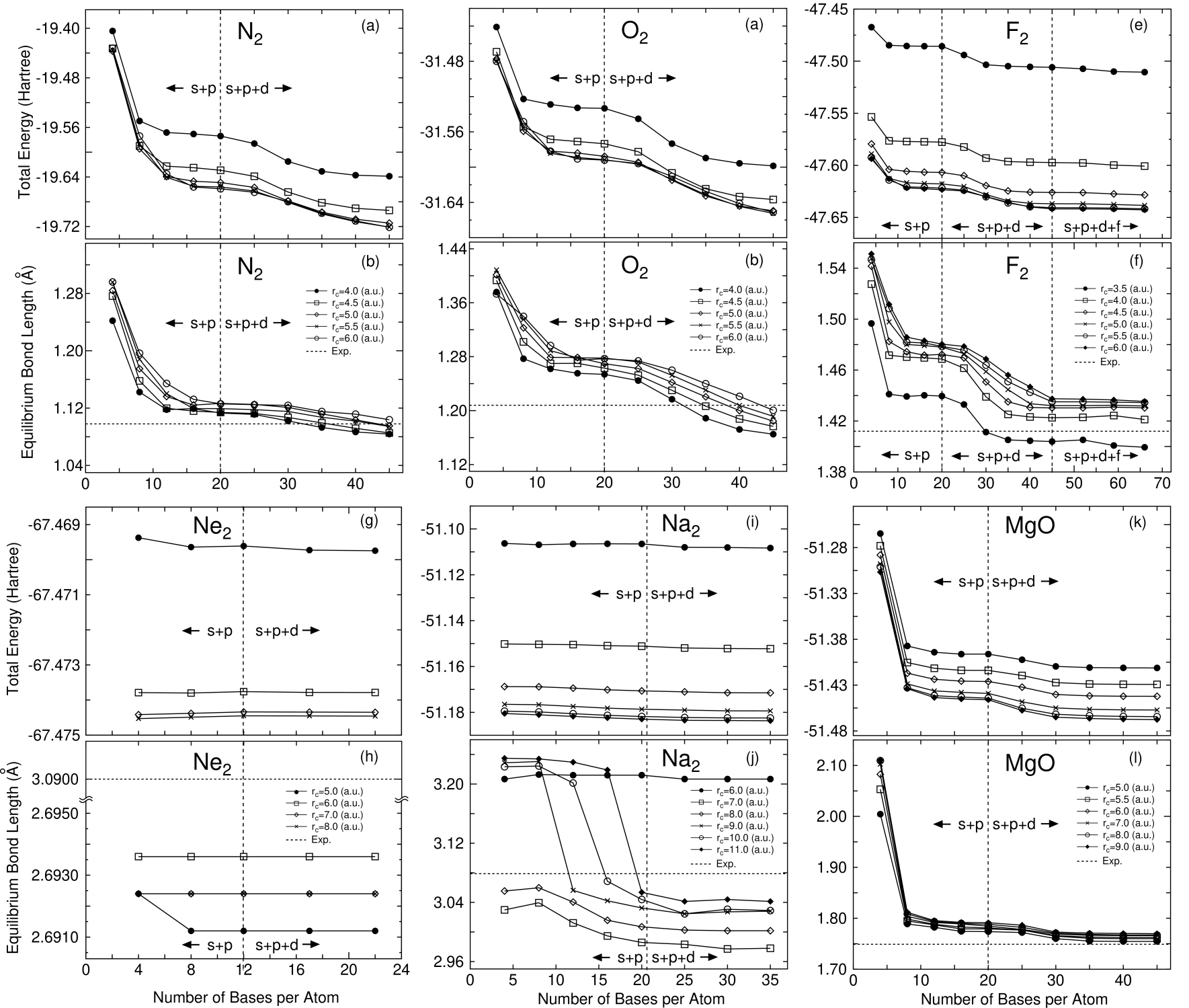
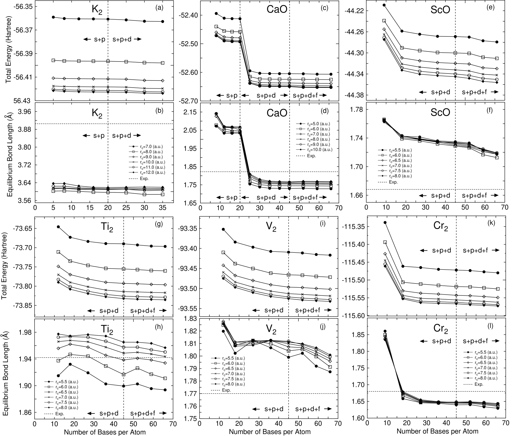
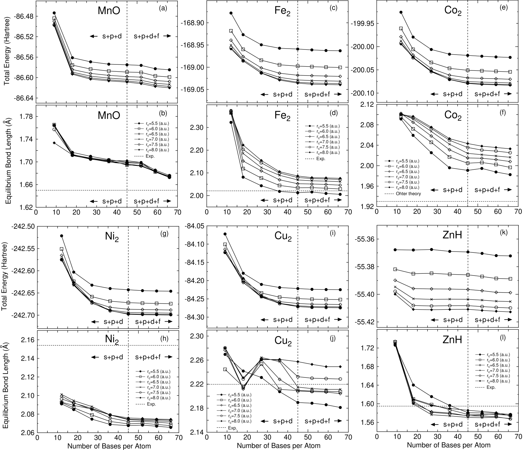
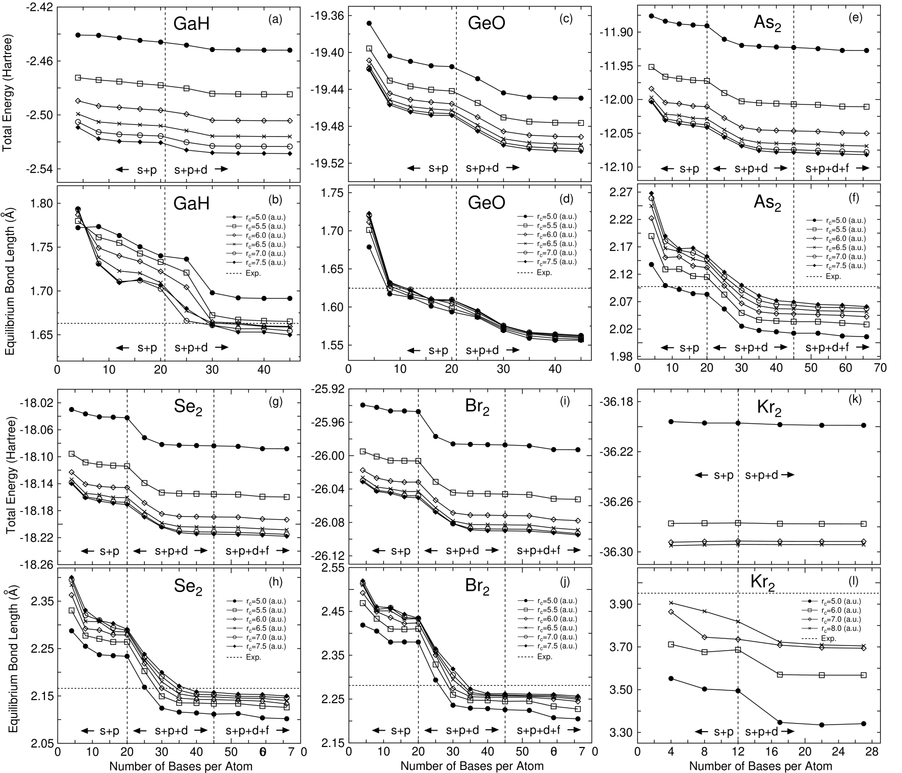
In Figs. 2-7 the total energies and the equilibrium bond lengths for dimer molecules from H to Kr are shown as a function of the number of primitive orbitals for various cutoff radii $r_{\rm c}$, where the total energies were calculated at the experimental bond length and the equilibrium bond lengths were computed by a cubic spline interpolation for the energy curve as a function of bond length. In most cases, a homonuclear diatomic molecule for each element was investigated. However, if the homonuclear diatomic molecule is not well resolved experimentally, or is highly weak binding, the monoxide or the monohydride was calculated instead of the homonuclear diatomic molecule. In our all DFT calculations, factorized norm conserving pseudo potentials[27,28] were used with multiple projectors proposed by Blochl.[29] In addition to valence electrons, semicore electrons were also considered in making of pseudo potentials for several elements such as alkaline, alkaline earth, and transition elements. Moreover, the nonlinear partial core correction (NLPCC)[30] was considered in the evaluation of the exchange-correlation terms except for a hydrogen and a helium atom. A relativistic correction was not included in the generation of pseudo potentials. The basis set superposition error (BSSE)[31] was not corrected, since the dissociation energy was beyond the scope of this paper. The electronic states and the cutoff radii used in the generation of these pseudo potentials[25] are shown in Table I, where the cutoff radii are given in parentheses. We limited the study within the local spin density approximation (LSDA)[32] to the exchange-correlation interactions, since we would like to focus our attention on the convergence properties with respect to the basis orbitals. Also the real space grid techniques were used with the energy cutoff given in the caption of figures in numerical integration[13] and the solution of Poisson's equation using the fast Fourier transformation (FFT). All calculations in this study were performed using our DFT code, OpenMX[25], which is designed for the realization of large scale calculations. We discuss the convergence properties with respect to the basis orbitals in the following categorized elements in Figs. 2-7.

Figure 6: The total energy and the equilibrium bond length of a manganese monoxide molecule MnO, an iron dimer Fe$_2$, a cobalt dimer Co$_2$, a nickel dimer Ni$_2$, a copper dimer Cu$_2$, and a zinc monohydride molecule ZnH as a function of the number of primitive basis orbitals per atom for different cutoff radii. The energy cutoff of 146, 146, 146, 146, 113, and 146 (Ryd) were used for the numerical integration and the solution of Poisson's equation in MnO, Fe$_2$, Co$_2$, Ni$_2$, Cu$_2$, and ZnH, respectively. In MnO and ZnH, we used 5.0 and 4.5 (a.u.) as a cutoff radius of primitive orbitals for the oxygen and hydrogen atoms, and increased the number of basis orbitals of the manganese, zinc, oxygen, and hydrogen atoms as Mnr$_{\rm c}$-smpmdmfn, Znr$_{\rm c}$-smpmdmfn, O5.0-smpmdn, and H4.0-smpn, where $r_{\rm c}$ is a cutoff radius, given in Figs. 6(b) and (l), of primitive orbitals for the manganese and zinc atoms. Exceptionally, a cobalt dimer was calculated, while the bond length of Co$_2$ determined experimentally is not available.

Figure 7: The total energy and the equilibrium bond length of a gallium monohydride molecule GaH, a germanium monoxide molecule GeO, an arsenic dimer As$_2$, a selenium dimer Se$_2$, a bromine dimer Br$_2$, and a krypton dimer Kr$_2$ as a function of the number of primitive basis orbitals per atom for different cutoff radii. The energy cutoff of 146, 146, 107, 107, 107, and 290 (Ryd) were used for the numerical integration and the solution of Poisson's equation in GaH, GeO, As$_2$, Se$_2$, Br$_2$, and Kr$_2$, respectively. In GaH and GeO, we used 4.5 and 5.0 (a.u.) as a cutoff radius of primitive orbitals for the hydrogen and oxygen atoms, and increased the number of basis orbitals of the gallium, germanium, hydrogen, and oxygen atoms as Gar$_{\rm c}$-smpmdn, Ger$_{\rm c}$-smpmdn, H4.0-smpn, and O5.0-smpmdn, where $r_{\rm c}$ is a cutoff radius, given in Figs. 7(b) and (d), of primitive orbitals for the gallium and germanium atoms.

Representative elements

In representative elements such as H, B, C, N, O, and F, systematic convergence properties are observed as expected. As the cutoff radius and the number of primitive orbitals increase, the total energy converges systematically. Along with the energy convergence, the calculated equilibrium bond length converges at the experimental value within an error of a few percentages. When the energy convergence is carefully observed from the left to the right elements in the first row, we find a trend that primitive orbitals with a higher angular momentum $l$ are required in order to achieve an enough convergence. Note that the primitive orbitals with a higher angular momentum $l$ beyond valence orbitals allocated to valence electrons are referred to as polarization orbitals according to quantum chemistry in this paper. In H$_2$ and C$_2$, the valence orbitals are almost enough to accomplish the energy convergence. The inclusion of polarization orbitals, $p$ and $d$ orbitals for hydrogen and carbon atoms, are not effective for the energy convergence. In N$_2$ and F$_2$, the total energies are significantly reduced by the inclusion of $d$ orbitals. The overestimated equilibrium bond lengths in the calculations by the $s$ and $p$ valence orbitals shorten in accordance with the inclusion of $d$ orbitals. The same trend as that observed in the first row is found in the convergence properties of the second row elements with respect to angular momentum of primitive orbitals. In P$_2$, S$_2$, and Cl$_2$ the polarization $d$ orbitals are relevant to obtain the convergent results, while the inclusion of the polarization $d$ orbitals insensibly decreases the total energy in Al$_2$ and Si$_2$. In the third row, the polarization $d$ orbitals are required in all representative elements from Ga to Br for the energy and geometrical convergences. If the valence $s$ and $p$ orbitals are only considered, the equilibrium bond lengths tend to be overestimated. Based on the calculations, rough estimations of appropriate cutoff radii of basis orbitals might be given as 5.0, 6.5, and 6.5 a.u. for representative elements of the first, the second, and the third rows, respectively. Although these rough estimations provide a practical guideline in an optimum choice of cutoff radius for each element, it should be mentioned that there is often an exceptional case in which a larger cutoff radius is required for the accurate description. As such an exceptional case, we can point out that a relatively larger cutoff radius must be used when an atom is negatively charged up, since the electrons tend to be far from the atom due to the repulsive interaction between electrons. In contrast, a smaller cutoff radius could be enough to achieve a sufficient convergence when an atom is positively charged up, and when an atom has a high coordination number which means that the atom is surrounded by the other many atoms. We will again discuss the cutoff radius in the later discussion based on numerical results.

TABLE II. The electronic configuration of the ground state predicted by our calculations within LSDA. The calculations were performed using experimental bond lengths, and the spin multiplicity are evaluated from the difference in Mulliken charges of up and down spins. The experimental ground states are also shown for comparison. The basis orbitals we used in these calculations are given in our basis specification in parentheses. For the oxygen and hydrogen atoms in all the monoxides and the monohydrides, O5.0-$s$2$p$2 and H4.5-$s$2 were used, respectively. For the energy cutoff we used the same values as those given in Figs. 2-7. The electronic configurations determined experimentally are taken from $^a$ Ref. [33], $^b$ Ref. [34], $^c$ Ref. [35], $^d$ Ref. [36], $^e$ Ref. [37], $^f$ Ref. [52], $^g$ Ref. [38], $^h$ Ref. [39], $^i$ Ref. [40], $^j$ Ref. [41], $^k$ Ref. [42], $^l$ Ref. [43], $^m$ Ref. [55], $^n$ Ref. [44], $^o$ Ref. [45], $^p$ Ref. [46], $^q$ Ref. [47], $^r$ Ref. [48], $^s$ Ref. [49], $^t$ Ref. [50], $^u$ Ref. [51], and $^v$ Ref. [53]. For Ni$_2$, the experiments [48] suggest the existence of a ground state with $\Omega=0_g^+$ or $0_u^-$, which would be a mixture of $^3\Sigma_g^-$ and $^1\Sigma_g^+ (0_g^-)$ or $^3\Sigma_u^+$ and $^1\Sigma_u^- (0_u^-)$.

Dimer	Expt.	Calc.	Dimer	Expt.	Calc.
H$_2$ (H4.5-$s$2)	$^1\Sigma_{\rm g}^+$ $^a$	$^1\Sigma_{\rm g}^+$ $(1s\sigma_g^2)$	K$_2$ (K10.0-$s$2$p$2)	$^1\Sigma_{\rm g}^+$ $^f$	$^1\Sigma_{\rm g}^+$ $(3p\pi_g^43p\sigma_u^24s\sigma_g^2)$
He$_2$ (He7.0-$s$2)	$^1\Sigma_{\rm g}^+$ $^b$	$^1\Sigma_{\rm g}^+$ $(1s\sigma_g^21s\sigma_u^2)$	CaO (Ca7.0-$s$2$p$2$d$2)	$^1\Sigma^+$ $^k$	$^1\Sigma^+$ $(s\sigma^2s\sigma^2p\pi^4)$
Li$_2$ (Li8.0-$s$2)	$^1\Sigma_{\rm g}^+$ $^c$	$^1\Sigma_{\rm g}^+$ $(2s\sigma_g^2)$	ScO (Sc7.0-$s$2$p$2$d$2)	$^2\Sigma^+$ $^l$	$^2\Sigma^+$ $(d\pi^4s\sigma^2s\sigma^1)$
BeO (Be6.0-$s$2$p$2)	$^1\Sigma^+$ $^d$	$^1\Sigma^+$ $(s\sigma^2s\sigma^2p\pi^4)$	Ti$_2$ (Ti7.0-$s$2$p$2$d$2)	$^3\Delta_g$ $^m$	$^3\Delta_g$ $(4s\sigma_g^23d\sigma_g^13d\pi_u^43d\delta_g^1)$
B$_2$ (B5.5-$s$2$p$2)	$^3\Sigma_{\rm g}^-$ $^e$	$^3\Sigma_{\rm g}^-$ $(2s\sigma_g^22s\sigma_u^22\pi_u^2)$	V$_2$ (V7.5-$s$2$p$2$d$2)	$^3\Sigma_g^-$ $^n$	$^1\Sigma_g^+$ $(4s\sigma_g^23d\sigma_g^23d\pi_u^43d\delta_g^2)$
C$_2$ (C5.0-$s$2$p$2)	$^1\Sigma_{\rm g}^+$ $^f$	$^1\Sigma_{\rm g}^+$ $(2s\sigma_g^22s\sigma_u^22p\pi_u^4)$	V$_2$ (V7.5-$s$4$p$4$d$4$f$2)	$^3\Sigma_g^-$ $^n$	$^3\Sigma_g^-$ $(4s\sigma_g^23d\sigma_g^23d\pi_u^43d\delta_g^2)$
N$_2$ (N5.0-$s$2$p$2)	$^1\Sigma_{\rm g}^+$ $^f$	$^1\Sigma_{\rm g}^+$ $(2s\sigma_u^22p\pi_u^42p\sigma_g^2)$	Cr$_2$ (Cr7.0-$s$2$p$2$d$2)	$^1\Sigma_g^+$ $^o$	$^1\Sigma_g^+$ $(4s\sigma_g^23d\sigma_g^23d\pi_u^43d\delta_g^4)$
O$_2$ (O5.0-$s$2$p$2)	$^3\Sigma_{\rm g}^-$ $^f$	$^3\Sigma_{\rm g}^-$ $(2p\sigma_g^22p\pi_u^42p\pi_g^2)$	MnO (Mn7.0-$s$2$p$2$d$2)	$^6\Sigma^+$ $^p$	$^6\Sigma^+$ $(d\sigma^1d\pi^4d\delta^2d\pi^{*2})$
F$_2$ (F5.0-$s$2$p$2)	$^1\Sigma_{\rm g}^+$ $^f$	$^1\Sigma_{\rm g}^+$ $(2p\sigma_g^22p\pi_u^42p\pi_g^4)$	Fe$_2$ (Fe7.0-$s$2$p$2$d$2)	$^7\Delta_u$ $^q$	$^7\Delta_u$ $(4s\sigma_g^23d\sigma_g^23d\sigma_u^13d\pi_u^43d\pi_g^23d\delta_g^33d\delta_u^2)$
Ne$_2$ (Ne7.0-$s$2$p$2)	$^1\Sigma_{\rm g}^+$ $^g$	$^1\Sigma_{\rm g}^+$ $(2p\pi_u^42p\pi_g^42p\sigma_u^2)$	Co$_2$ (Co7.0-$s$2$p$2$d$2)		$^5\Delta_g$ $(4s\sigma_g^23d\sigma_g^23d\sigma_u^13d\pi_u^43d\pi_g^23d\delta_g^43d\delta_u^3)$
Na$_2$ (Na9.0-$s$2$p$2)	$^1\Sigma_{\rm g}^+$ $^f$	$^1\Sigma_{\rm g}^+$ $(2p\pi_g^42p\sigma_u^23s\sigma_g^2)$	Ni$_2$ (Ni7.0-$s$2$p$2$d$2)	$\Omega$ $^r$	$^3\Sigma_g^-$ $(4s\sigma_g^23d\sigma_g^23d\sigma_u^23d\pi_u^43d\pi_g^23d\delta_g^43d\delta_u^4)$
MgO (Mg7.0-$s$2$p$2)	$^1\Sigma^+$ $^h$	$^1\Sigma^+$ $(s\sigma^2s\sigma^2p\pi^4)$	Cu$_2$ (Cu7.0-$s$2$p$2$d$2)	$^1\Sigma_g^+$ $^s$	$^1\Sigma_g^+$ $(4s\sigma_g^23d\sigma_g^23d\sigma_u^23d\pi_u^43d\pi_g^43d\delta_g^43d\delta_u^4)$
Al$_2$ (Al6.5-$s$2$p$2)	$^3\Pi_{\rm u}$ $^i$	$^3\Sigma_{\rm g}^-$ $(3s\sigma_g^23s\sigma_u^23p\pi_u^2)$	ZnH (Zn7.0-$s$2$p$2$d$2)	$^2\Sigma_g^+$ $^t$	$^2\Sigma_g^+$ $(s\sigma^2s\sigma^{*1}d\sigma^2d\pi^4d\delta^4)$
Al$_2$ (Al6.5-$s$4$p$4$d$2)	$^3\Pi_{\rm u}$ $^i$	$^3\Sigma_{\rm g}^-$ $(3s\sigma_g^23s\sigma_u^23p\pi_u^2)$	GaH (Ga7.0-$s$2$p$2)	$^1\Sigma^+$ $^u$	$^1\Sigma^+$ $(s\sigma^2s\sigma^{*2})$
Si$_2$ (Si6.5-$s$2$p$2)	$^3\Sigma_{\rm g}^-$ $^f$	$^3\Pi_{\rm u}$ $(3s\sigma_u^23s\sigma_g^13p\pi_u^3)$	GeO (Ge7.0-$s$2$p$2)	$^1\Sigma^+$ $^f$	$^1\Sigma^+$ $(ss\sigma^2sp\sigma^{2}pp\pi^4pp\sigma^2)$
Si$_2$ (Si6.5-$s$2$p$2$d$1)	$^3\Sigma_{\rm g}^-$ $^f$	$^3\Sigma_{\rm g}^-$ $(3s\sigma_u^23p\pi_u^23s\sigma_g^2)$	As$_2$ (As7.0-$s$2$p$2$d$1)	$^1\Sigma^+_g$ $^f$	$^1\Sigma^+_g$ $(4s\sigma^2_g4s\sigma^2_u4p\sigma_g^24p\pi^4_u)$
P$_2$ (P6.0-$s$2$p$2$d$1)	$^1\Sigma_{\rm g}^+$ $^f$	$^1\Sigma_{\rm g}^+$ $(3s\sigma_u^23p\sigma_g^23p\pi_u^4)$	Se$_2$ (Se7.0-$s$2$p$2$d$1)	$^3\Sigma^-_g$ $^f$	$^3\Sigma^-_g$ $(4s\sigma^2_g4s\sigma^2_u4p\sigma_g^24p\pi^4_u4p\pi_g^2)$
S$_2$ (S6.0-$s$2$p$2)	$^3\Sigma_{\rm g}^-$ $^f$	$^3\Sigma_{\rm g}^-$ $(3p\sigma_g^23p\pi_u^43p\pi_g^2)$	Br$_2$ (Br7.0-$s$2$p$2$d$1)	$^1\Sigma^+_g$ $^f$	$^1\Sigma^+_g$ $(4s\sigma^2_g4s\sigma^2_u4p\sigma_g^24p\pi^4_u4p\pi_g^4)$
Cl$_2$ (Cl6.0-$s$2$p$2$d$2)	$^1\Sigma_{\rm g}^+$ $^f$	$^1\Sigma_{\rm g}^+$ $(3p\sigma_g^23p\pi_u^43p\pi_g^4)$	Kr$_2$ (Kr7.0-$s$2$p$2)	$^1\Sigma^+_g$ $^v$	$^1\Sigma^+_g$ $(4s\sigma^2_g4s\sigma^2_u4p\sigma_g^24p\sigma_u^24p\pi^4_u4p\pi_g^4)$
Ar$_2$ (Ar7.0-$s$2$p$2)	$^1\Sigma_{\rm g}^+$ $^j$	$^1\Sigma_{\rm g}^+$ $(3p\pi_u^43p\pi_g^43p\sigma_u^2)$

Moreover, the convergence with respect to the basis orbitals could be confirmed when the electronic state is carefully examined. In Table II, we find that the electronic configurations of the experimental ground state are well reproduced in the first row representative elements by only the inclusion of valence orbitals. However, the polarization orbitals are more important for the second and third row elements to obtain a convergent result in the electronic configuration. Actually, the use of only the valence orbitals fails to predict the ground state of Si$_2$. The basis orbitals, Si6.5-$s$2$p$2, gives $^3\Pi_u$ to be the ground state of Si$_2$, while the ground state is correctly predicted as $^3\Sigma_g^-$ by the inclusion of $d$ orbitals. Although the ground state of Al$_2$ is determined as $^3\Sigma_g^-$, even if the $d$ orbitals are included, experimental investigations reveal that the ground state is $^3\Pi_g^-$.[40] The discrepancy between our theoretical prediction and the experiments is attributed to LSDA to the exchange-correlation interaction as reported by Martinez et al.[66] They also obtained $^3\Sigma_g^-$ as the ground state of Al$_2$ within LSDA, while their GGA calculation correctly predicts that the ground state of Al$_2$ is $^3\Pi_g^-$ and the $^3\Sigma_g^-$ state is the lowest excited state.[66] For the third row representative elements, we did not observe the same kind of discrepancy as that of Si$_2$ in prediction of the ground state. However, the inclusion of $d$ orbitals is recommended for the geometrical convergence as mentioned before. Table III enumerated the equilibrium bond lengths which are calculated using the orbitals with the largest cutoff radius and the greatest number of orbitals for each dimer in Figs. 2-7. The calculated bond lengths of dimer molecules by representative elements are consistent with both the experimental and the other theoretical values, which supports that our primitive basis orbitals provide the convergent results comparable to the other DFT calculations.

Transition elements

As well as the representative elements, we find systematic convergence properties with respect to the cutoff radius and the number of primitive orbitals for the first row transition elements. Both the total energy and equilibrium bond length converge with increasing of the cutoff radius of orbitals and the number of orbitals. Interestingly, the polarization $f$ orbitals do not play an important role in the energy convergence. Within the valence orbitals the energy convergence is almost achieved in all the transition elements that we considered. However, there would be a possibility that the polarization orbitals become more effective for transition elements in a higher row which lies downward in the periodic table we have not studied, like the representative elements. In Table II, we find that the predicted electronic configurations of the ground states are almost consistent with the experimental results within the use of only valence orbitals, except for V$_2$ and Ni$_2$. In V$_2$ the electronic configuration, $^3\Sigma_g^+$, observed experimentally[44] is correctly reproduced by the inclusion of the polarization $f$ orbitals, while only the use of the valence orbitals predicts $^1\Sigma_g^+$ as the ground state of V$_2$. The non-monotonic convergence of the equilibrium bond length of V$_2$ found in Fig. 5 can be attributed to the transition of singlet to triplet in the calculated ground state. For Ni$_2$, recent experiments[48] by resonant two-photon ionization spectroscopy using argon carrier gas suggest that the ground state is $\Omega=0_g^+$ or $0_u^-$, which would be a mixture of $^3\Sigma_g^-$ and $^1\Sigma_g^+ (0_g^-)$ or $^3\Sigma_u^+$ and $^1\Sigma_u^- (0_u^-)$. In contrary, we obtained $^3\Sigma_g^-$, which is a $\pi\pi$ hole state, as the ground state within LSDA. Although the calculated ground state $^3\Sigma_g^-$ is not consistent with the experiments[48], but is equivalent to the other theoretical prediction[70] within generalized gradient approximations (GGA) to the exchange-correlation interaction. Thus, the discrepancy between the theoretical prediction and the experiments must be attributed to the poor description to exchange-correlation interaction or the limitation of single configuration method such as DFT rather than the quality of basis orbitals. Also, in Table III we see that the calculated bond lengths are comparable to both the experimental and the other theoretical values. For the first row transition elements, a rough estimation of appropriate cutoff radius of basis orbitals might be given as 7.0 a.u. based on the calculations of dimer molecules, which provides a trade-off between the computational accuracy and efficiency. However, as discussed in the representative elements, it should be noted that the appropriate choice of cutoff radius depends on atomic environments and states such as the coordination number and the charge state.

TABLE III. The calculated equilibrium bond lengths which are calculated using the orbitals with the largest cutoff radius and the greatest number of orbitals for each dimer in Figs. 2-7. The experimental bond lengths and the other theoretical values are also shown for comparison, which are taken from $^A$ Ref. [52], $^B$ Ref. [53], $^C$ Ref. [54], $^D$ Ref. [55], $^E$ Ref. [56], $^F$ Ref. [57], $^G$ Ref. [58], $^H$ Ref. [59], $^I$ Ref. [60], $^a$ Ref. [61], $^b$ Ref. [62], $^c$ Ref. [63] (B3LYP), $^d$ Ref. [64] (APW), $^e$ Ref. [20], $^f$ Ref. [65], $^g$ Ref. [66], $^h$ Ref. [67], $^i$ Ref. [68] (BLYP), $^j$ Ref. [69] (PW86-P86), $^k$ Ref. [70] (PW91), $^l$ Ref. [72], $^m$ Ref. [73], $^n$ Ref. [74], For a substantial comparison between our calculations and the other theoretical results, the other calculations based on pseudo potentials and LSDA are listed. In case of the lack of calculations at the same level, computational results performed with the other context are listed, of which method is denoted in parentheses in this caption.

	Expt.	Present	Other		Expt.	Present	Other
H$_2$	0.741$^A$	0.768	0.766$^a$	K$_2$	3.905$^A$	3.620	3.670$^a$
He$_2$	2.97 $^B$	2.417	2.397$^b$	CaO	1.822$^A$	1.768	1.79$^f$
Li$_2$	2.673$^A$	2.748	2.699$^a$	ScO	1.668$^A$	1.719	1.649$^a$
BeO	1.331$^A$	1.339	1.319$^c$	Ti$_2$	1.942$^D$	1.957	-
B$_2$	1.590$^A$	1.603	-	V$_2$	1.77 $^E$	1.801	1.802$^j$
C$_2$	1.243$^A$	1.255	1.249$^d$	Cr$_2$	1.679$^F$	1.643	1.632$^k$
N$_2$	1.098$^A$	1.104	1.094$^a$	MnO	1.648$^G$	1.673	1.585$^a$
O$_2$	1.208$^A$	1.201	1.197$^e$	Fe$_2$	2.02 $^H$	2.076	1.963$^l$
F$_2$	1.412$^A$	1.435	1.388$^a$	Co$_2$	-	2.033	1.93$^m$
Ne$_2$	3.09 $^B$	2.692	2.641$^b$	Ni$_2$	2.155$^I$	2.074	2.037$^n$
Na$_2$	3.079$^A$	3.140	3.048$^a$	Cu$_2$	2.220$^A$	2.249	2.170$^n$
MgO	1.749$^A$	1.770	1.76$^f$	ZnH	1.595$^A$	1.574	1.593$^a$
Al$_2$	2.650$^C$	2.710	2.73$^g$	GaH	1.663$^A$	1.650	1.681$^a$
Si$_2$	2.246$^A$	2.281	2.280$^h$	GeO	1.625$^A$	1.563	1.593$^a$
P$_2$	1.893$^A$	1.926	1.877$^a$	As$_2$	2.103$^A$	2.066	2.070$^a$
S$_2$	1.889$^A$	1.936	1.942$^i$	Se$_2$	2.166$^A$	2.150	2.164$^a$
Cl$_2$	1.987$^A$	1.946	1.971$^a$	Br$_2$	2.281$^A$	2.257	2.273$^a$
Ar$_2$	3.76 $^B$	3.425	3.42$^b$	Kr$_2$	3.951$^B$	3.705	3.715$^b$

Figure 8: The pseudo radial wave functions of 4$s$ orbital in potassium, iron, and bromine atoms, which are generated by the TM scheme. For ease of comparison, the 3$s$ semicore state of potassium atom was excluded in the pseudo potential generation to make the 4$s$ orbital nodeless, while the 3$s$ semicore state was considered in Table I. For iron and bromine atoms, the pseudo wave functions were calculated under the same conditions as shown in Table I.

Figure 9: The total energy, equilibrium lattice constant, bulk modulus, and magnetic moment of carbon and silicon in the diamond, gallium arsenide in the zinc blend, carbon in the graphite, and the bcc iron as a function of the number of primitive basis orbitals per atom for different cutoff radii, in which the energy cutoff of 168, 120, 120, 156, and 170 (Ryd) were used for the numerical integration and the solution of Poisson's equation, respectively. The bulk modulus was calculated by a least square fitting of the total energy curve to Murnaghan's equation of state.[75] The magnetic moment in the bcc iron are evaluated from the difference in Mulliken charges of up and down spins. In the graphite carbon, the lattice constant of only the $ab$ plane was varied with a lattice constant of the $c$ axis fixed at the experimental value. The lack of datum calculated using Fe4.5-$s$3$p$3$d$3 or more in Figs. 9(l)-(o) is due to the overcompleteness of basis orbitals as discussed in context.

Alkaline and alkaline earth elements

Intrinsically, it would be hard to describe KS orbitals of systems consisting of alkaline and alkaline earth elements by using LCAO with short range atomic orbitals. In Fig. 8 shows nodeless pseudo radial wave functions of $4s$ state in K, Fe, and Br atoms, which are generated by the pseudo potential calculations. The comparison definitely reveals that the radial wave function of an alkaline element has a longer tail compared to those of a transition element and a representative element, which might make the use of basis orbitals with a short cutoff radius difficult. Actually, we find in Figs. 2-7 that a large cutoff radius is required for dimer molecules of alkaline elements to achieve a sufficient convergence in the total energy and the equilibrium bond length. At least 9.0, 9.0, and 10.0 a.u. of the cutoff radii are needed for Li, Na, and K atoms, respectively. It should be noted that the requirement of a larger cutoff radius for alkaline elements causes great computational demands in the evaluation of the Hamiltonian matrix elements, since the number of grids in the sphere defined with a cutoff radius $r_c$ scales as O($r_c^3$). In contrast, the energy dependency on the number of orbitals is not so large, which represents that the convergence is almost accomplished even if a small number of orbitals are employed. This energy independency with respect to number of orbitals helps us to reduce the computational costs in the application of LCAO to alkaline metal systems in spite of the requirement of a large cutoff radius. For alkaline earth elements, the monoxide molecules were investigated for ease of calculations, since accurate calculations require a considerably larger cutoff energy for the numerical integration and the solution of Poisson's equation due to highly weak binding of the homonuclear diatomic molecules of alkaline earth elements. From Figs. 2-7 we find that the total energies and the equilibrium bond length systematically converge as the cutoff radius and the number of primitive orbitals increase like representative elements. In these monoxide molecules, 7.0 a.u. of the cutoff radius gives a trade-off between the computational accuracy and efficiency for all the alkaline earth elements. The inclusion of polarization $d$ oribtals is essential for the convergence in CaO, while the $d$ orbitals do not play an important role in the energy and geometrical convergences of BeO and MgO. This is because the $3d$ state of a calcium atom exists near the valence $4s$ state. Therefore, the $3d$ orbitals of CaO considerably contribute in $\sigma$ and $\pi$ KS orbitals. In fact, the LCAO coefficient of the $d_{xy}$ orbital with a nodeless radial function of the calcium atom is about 0.3 in the occupied $\pi$ orbital of the monoxide molecule along $x$ axis, in which Ca7.0-$s$2$p$2$d$2 and O5.0-$s$2$p$2 were used as the basis orbitals. In Table II gives the electronic configurations for the ground state of the alkaline element dimers and the monoxide molecules of alkaline earth elements. The calculated electronic configurations for the ground state are wholly consistent with those determined experimentally. Also, we find in Table III that the calculated equilibrium bond lengths are comparable to both the experimental and the other theoretical values for the alkaline element dimers and the monoxide molecules of alkaline earth elements. These results support that our primitive basis orbitals give a complete basis set even for the alkaline and alkaline earth elements, while the cutoff radius required for the convergence is larger than those of representative and transition elements.

Rare gas elements

It has been reported that LDA and GGA fail to predict the equilibrium bond lengths and the dissociation energies of dimer molecules consisting of rare gas elements weakly binding by Van der Waals interactions.[62] However, our attention in this study is to know the convergence properties with respect to basis orbitals. Therefore, we investigated homonuclear diatomic molecules of rare gas elements, He, Ne, Ar, and Kr within LDA, and compared the calculated equilibrium bond lengths with the other theoretical values calculated by LDA. The dissociation energies of the rare gas dimers are significantly small unlike dimers of representative and transition elements. Therefore, we had to use higher cutoff energies, which are 262, 343, 290, and 290 (Ryd) for He$_2$, Ne$_2$, Ar$_2$, and Kr$_2$, for the numerical integration and the Poisson's equation so that the computations are not buried in numerical errors. It seems that the convergence in the total energy of rare gas dimers depends on only the cutoff radius of primitive orbitals. For all the rare gas dimers 7.0 a.u. of the cutoff radius are enough to accomplish a sufficient convergence. On the other hand, the calculated equilibrium bond lengths have a dependency on the number of orbitals, especially in Ar$_2$ and Kr$_2$, however, the double valence with single polarization orbitals provide almost convergence results even for Ar$_2$ and Kr$_2$. In Table III we see that the calculated equilibrium bond lengths are comparable to the other theoretical values calculated by all electron calculations within LDA. In addition, the calculated electronic configurations for the ground states are consistent with those reported experimentally. Thus, our primitive orbitals could be a systematic basis set for rare gas dimers as well as representative, transition, and alkaline and alkaline earth elements, while the Van der Waals interactions in the rare gas dimers is not correctly taken into account in LDA calculations.

Bulks

For selected bulk systems, we investigated the convergence properties of total energy, lattice constant, bulk modulus, and magnetic moment with respect to basis orbitals as shown in Fig. 9. The bulk modulus was calculated by a least square fitting of the total energy curve to Murnaghan's equation of state.[75] The magnetic moment in the bcc iron are evaluated from the difference in Mulliken charges of up and down spins. In the graphite carbon, the lattice constant of only the $ab$ plane was varied with a lattice constant of the $c$ axis fixed at the experimental value. For all bulk systems the same systematic convergence as that for dimer molecules is achieved as the cutoff radius and the number of primitive orbitals increase. When the shorter cutoff radius of primitive orbitals was used, the calculated lattice constant (bulk modulus) tend to be shorter (greater) than the experimental values. As the cutoff radius increases, these calculated values converge at experimental values within an error of a few percentages. For carbon in the diamond and graphite, 4.0 and 4.5 a.u. of the cutoff radius might be regarded as a trade-off between the computational accuracy and efficiency, respectively. The comparison in an appropriate cutoff radius for various systems suggests that the coordination number of each atom is an important factor which determines an adequate values of the cutoff radius. Our rough estimations of an appropriate cutoff radius are 5.0, 4.5, and 4.0 a.u. for the carbon dimer C$_2$, the diamond carbon, and the graphite carbon of which the coordination numbers are one, three, and four. Thus, an appropriate cutoff radius could be in inverse proportion to the coordination numbers. This observation is also confirmed in a comparison of the convergence with respect to a cutoff radius for iron, an iron dimer Fe$_2$ and the bcc iron. In the bcc iron, we can obtain almost convergent results using 4.5 a.u. of the cutoff radius, while 7.0 a.u. are needed to obtain the convergence in Fe$_2$.

Here, it must be stressed that the calculation of the bcc iron illustrates a limitation in applicability of LCAO method. We found that it was difficult to perform reliable calculations of the bcc iron using Fe4.5-$s$3$p$3$d$3 or more. In particular, it was unable to perform meaningful calculations due to numerical errors for the bcc iron with a shorter lattice parameter. The problem comes from the overcompleteness of basis orbitals. In the bcc iron with a shorter lattice parameter and the use of a longer cutoff radius of basis orbitals, eigenvalues of the overlap matrix can be negative, which means that the basis orbitals is not linearly independent. A remedy in this case is to reduce matrices by removing eigenvectors corresponding to the negative eigenvalues. However, the eigenvalues of the overlap matrix in bulk systems distribute continuously as a function of energy, thus, many ill-conditioned eigenvalues, which are positive but almost zero, appear in the eigenvalue spectrum. The division by the ill-conditioned eigenvalues brings about the numerical instability we met. If basis orbitals with a larger cutoff radius is used for a dense system with atoms of large coordination numbers, a small number of optimized orbitals should be used to avoid the numerical instabilities.

IV. VARIATIONAL OPTIMIZATION

In this Section, we present a simple and practical method for variationally optimizing numerical basis orbitals of each atom located on different environments in a given system.[16] Starting from the primitive basis orbitals discussed in the Sec. II, the shape of radial wave functions of each atom are variationally optimized within a given cutoff radius so that the total energy is minimized based on the force theorem. The orbital optimization scheme promises us to reduce the computational cost, while keeping a high degree of accuracy. Although the primitive radial wave function $R'_{ipl}$, the eigenstate of atomic KS equation with a confinement potential, was used as radial basis orbital $R_{ipl}$ of the KS orbital in a form of LCAO in Sec. II, here, we reconsider a different expression for $R_{ipl}$ and thus $\phi_{i\alpha}$. To give a variational degree of freedom of $\phi_{i\alpha}$, we furthermore expand $\phi_{i\alpha}$ using primitive orbitals $\chi_{i\eta}(\equiv Y_{lm}R'_{iql})$ as follows:

$$\phi_{i\alpha}({\bf r}) = \sum_{q} a_{iplm q} Y_{lm}R'_{iql},$$

$$= \sum_{q} a_{i\alpha q} \chi_{i\eta}({\bf r}),$$ (3)

where $\eta\equiv (qlm)$, in which the indices $l$ and $m$ denote the same as those of the index $\alpha$. Note that a primitive radial wave function $R'_{iql}$ is independent on $m$, and that the coefficients $a_{i\alpha q}$ are independent variables on the eigenstate $\mu$, but could depend on a magnetic quantum number $m$. Therefore, we prefer the expression Eq. (3), which is expanded by a linear combination of $\chi_{i\eta}$, rather than a expansion by the primitive radial function $R'_{ipl}$ itself. The expression Eq. (3) is similar to a contraction used in quantum chemistry based on Gaussian orbitals, in which basis orbitals are expanded by a linear combination of several Gaussian orbitals. Therefore, the basis orbital by the expression Eq. (3) will be referred to as contracted orbital or optimized orbital. For the later discussion, we moreover extend the abbreviation introduced in Sec. II to the contracted orbital by Eq. (3) as C4.5-$s$62$^*$$p$62, where C indicates the atomic symbol, 4.5 is the cutoff radius $r_{\rm c}$ (a.u.) used in the generation as well as discussed in Sec. II, $s$62 means that two optimized orbitals are constructed from six primitive orbitals for the $s$ orbital, and the symbol $^*$ signifies the restricted optimization that the radial wave function $R$ is independent on the index $m$. In case of $s$nn such as $s$66, corresponding to no optimization, $s$nn can be simplified as $s$n, which is equivalent to the abbreviation introduced in Sec. II.

Figure 10: The total energy for a carbon dimer C$_2$, a methane molecule CH$_4$, carbon and silicon in the diamond structure, a ethane molecule C$_2$H$_6$, and a hexafluoro ethane molecule C$_2$F$_6$ as a function of the number of primitive and optimized orbitals. The total energy and the number of orbitals are defined as those per atom for C$_2$, carbon and silicon in the diamond, and as those per molecule for CH$_4$, C$_2$H$_6$, and C$_2$F$_6$. The energy cutoff of 113, 113, 222, 120, 120, and 120 (Ryd) were used for the numerical integration in C$_2$, CH$_4$, carbon and silicon in the diamond structure, C$_2$H$_6$, and C$_2$F$_6$, respectively. The two step convergence of C$_2$ is due to the inclusion of polarization $d$ orbitals, where the basis specification was C4.5-$s$m$p$m$d$n and C4.5-$s$6m$p$6m$d$6n for the primitive and optimized orbitals, respectively. In the other system, only the valence $s$ and $p$ orbitals were used, where the basis specifications are as follows: in CH$_4$ H4.0-$s$m, C4.5-$s$m$p$m, and H4.0-$s$6m, C4.5-$s$6m$p$6m for the primitive and optimized orbitals, respectively, in carbon in the diamond C4.5-$s$m$p$m and C4.5-$s$5m$p$5m for the primitive and optimized orbitals, respectively, in silicon in the diamond Si6.5-$s$m$p$m and Si6.5-$s$5m$p$5m for the primitive and optimized orbitals, respectively, in C$_2$H$_6$ H4.5-$s$m, C5.0-$s$m$p$m, and H4.5-$s$5m, C5.0-$s$6m$p$6m for the primitive and optimized orbitals, respectively, in C$_2$F$_6$ C5.0-$s$m$p$m, F5.0-$s$m$p$m, and C5.0-$s$5m$p$5m, C5.0-$s$5m$p$5m for the primitive and optimized orbitals, respectively.

The contraction coefficients $a_{i\alpha q}$ can be easily optimited by the two step optimization scheme. The details of the two step optimization scheme has already been described in elsewhere [16]. In this two step optimization scheme, the atomic orbitals are optimized variationally in the same two step procedure as that of the geometry optimization in terms of $a_{i\alpha q}$ instead of atomic positions. The radial parts of basis orbitals in each atom located on different environment are automatically varied so that the total energy is minimized, which is a quite important advantage of our scheme compared to the other optimization method [12,13]. In the later part of this section, we demonstrate capability of our method based on numerical results. Figure 10 shows the convergence properties of total energies for a carbon dimer C$_2$, a methane molecule CH$_4$, carbon and silicon in the diamond structure, an ethane molecule, and a hexafluoro ethane molecule as a function of the number of primitive and optimized orbitals. The orbital optimization was done by ten iterative steps according to Eq. (7), in which each step includes ten SCF loops on the average. We see that the unoptimized orbitals provide systematic convergent results for not only molecules, but also bulk systems as the number of orbitals increase as discussed in Sec. II. Moreover, remarkable convergent results are obtained using the optimized orbitals for all systems. The small set of optimized orbitals rapidly converge to the total energies calculated by a larger number of the primitive orbitals, which implies that the computational effort can be reduced significantly with a high degree of accuracy. Only the restricted contraction was investigated in this study, since we found in the previous study that the unrestricted optimization is not effective to minimize the total energy.[16] Also, the restricted optimization guarantees the rotational invariance of the total energy. Therefore, our study was limited within the restricted optimization.

In Fig. 4 the radial parts of the minimal orbitals obtained by the restricted optimization for C$_2$H$_6$ and C$_2$F$_6$ are shown with those of the lowest primitive orbitals of an carbon atom for comparison. It is observed that the tails of both the optimized $s$ and $p$ orbitals shrink compared to the primitive orbitals in C$_2$H$_6$ and C$_2$F$_6$. In addition, we find that the $p$ orbitals of the carbon atom in C$_2$F$_6$ more shorten than that of C$_2$H$_6$. The considerable shortening tail of the $p$ orbital is related to change in the effective charge of carbon atom. Decomposed Mulliken populations of the carbon atom are 1.05 and 2.67 in C$_2$H$_6$, and 0.86 and 2.00 in C$_2$F$_6$ for $s$ and $p$ orbitals, respectively. So, we see that the deviation for the $p$ orbital is larger than that for the $s$ orbital in a comparison of the decomposed Mulliken population. Therefore, the large shortening tail of $p$ orbital in C$_2$F$_6$ is due to increase of effective core potential for $p$ electrons. The comparison between C$_2$H$_6$ and C$_2$F$_6$ clearly reveals that the shape of the basis orbital can automatically vary within the cutoff radius in order to respond to the change of the environment of each atom, while minimizing the total energy.

Figure 11: The radial wave function of the minimal orbitals of the carbon atom obtained by the restricted orbital optimization for a ethane molecule C$_2$H$_6$ and a hexafluoro ethane molecule C$_2$F$_6$, and the lowest primitive orbitals of a carbon atom. The optimization was done in the same conditions as those in Fig. 10.

Finally, as illustrations of the orbital optimization, we demonstrate two examples: the geometry optimization coupled with the orbital optimization of a C$_{60}$ molecule and the pre-orbital optimization for a set of amino acid residues.

First, we performed the geometry optimization with the orbital optimization as a preconditioning for a C$_{60}$ molecule. Before doing the geometry optimization, the orbital optimization was performed by ten iterative steps, which includes ten SCF loops per step on the average.

TABLE IV. Optimized geometrical parameters (Å and degrees) of a C$_{60}$ molecule. The computational time per MD step was measured using one Pentium 4 processor (2.8 GHz). The energy cutoff of 108 (Ryd) was used for the numerical integration in all calculations. The results by the other theory were taken from Ref. [80], and the experimental values from Ref. [81].

	SN	TN	TNDP	SN$'$	SNP$'$	Other theory	Expt.
	C4.5-$s$1$p$1	C4.5-$s$3$p$3	C4.5-$s$3$p$3$d$2	C4.5-$s$31$^*$$p$31$^*$	C4.5-$s$31$^*$$p$31$^*$$d$21$^*$
$r$(C$=$C)	1.439	1.391	1.393	1.395	1.393	1.39-1.41	1.40
$r$(C$-$C)	1.489	1.455	1.448	1.452	1.447	1.44-1.45	1.45
(C$-$C$-$C)	108.0	108.0	108.0	108.0	108.0	108.0	-
(C$=$C$-$C)	120.0	120.0	120.0	120.0	120.0	120.0	-
Energy (Hartree)	-333.729	-336.432	-336.939	-335.513	-336.233	-	-
Time(s)/MD step	168	403	1680	191	339	-	-

Then, the geometry optimization was done using the optimized orbitals by fifty steepest decent (SD) steps with a variable prefactor for accelerating the convergence, which includes fourteen SCF loops per step on the average. The optimized geometrical parameters are given in Table IV together with the total energy and the computational time per MD step. In case of the unoptimized primitive orbitals SN, TN, and TNDP, as the number of orbitals increase, we find the decrease of the total energy and the convergent geometrical parameters comparable to the experimental and the other theoretical values. Comparing to the unoptimized primitive and optimized minimal orbitals SN and SN$'$, it is found that the geometrical parameters calculated using SN$'$ are significantly improved without increasing the computational time. In case of the optimized orbitals SNP$'$, a complete convergence, which is comparable to TNDP, is achieved in the geometrical parameters with a great reduction of the computational time. The comptuational time required for the orbital optimization of SN$'$ occupies only 4 % of that of the whole calculation. So the orbital optimization can be utilized as a preconditioning before doing the geometry optimization or the molecular dynamics. Of course, it is possible to perform the orbital optimization during the geometry optimization for further accuracy. It is worth mentioning that the orbital optimization can be combined with an O($N$) method [6,7,8,9,10,11], since only $\Theta_{i\alpha, j\beta}$ and $E_{i\alpha, j\beta}$, which are calculated by the O($N$) method, are required in Eq. (6). Therefore, the orbital optimization can be applied to large scale systems in O($N$) operations.

Second, we show that it is significantly effective for the realization of a high degree of accuracy and efficiency to construct a database of optimized orbitals for a specific group such as proteins. Proteins are constructed from twenty kinds of amino acid residues. So, we categorized atoms in the residues as eleven, eighteen, four, three, and two kinds of hydrogen, carbon, nitrogen, oxygen, and sulfur atoms from a chemical point of view in consideration of chemical environment and connectivity. To construct a database of optimized orbitals for the categorized atoms, the structures of tripeptides, Gly-X-Gly, are considered for the orbital optimization, where X could be one of twenty kinds of amino acid residues. The structure of a Gly-X-Gly was optimized by a molecular mechanics (MM) using a software TINKER[85] with a AMBER98 force field[86] before the orbital optimization. Then, for the optimized Gly-X-Gly the restricted orbital optimization was performed by ten iterative steps with nine SCF loops per step on the average, in which LDA was employed to exchange-correlation interaction and the cutoff energy of 130 Ryd was used for numerical integration and the solution of Poisson's equation. In a series of optimizations, the basis specifications were given as H4.5-$s$52$^*$$p$51$^*$, C5.0-$s$52$^*$$p$52$^*$$d$51$^*$, N4.5-$s$52$^*$$p$52$^*$$d$51$^*$, O4.5-$s$52$^*$$p$52$^*$$d$51$^*$, and S6.0-$s$52$^*$$p$52$^*$$d$51$^*$. Because of the basis specifications, the orbitals stored in the database are well optimized for the use of double valence plus polarization orbitals. However, the basis sets maybe provide a better performance even for the other specifications of basis sets compared to the original primitive basis sets, when the basis sets are used for calculations of proteins. Following the construction of the database, we performed SCF calculations of small polypeptides to investigate the transferability of the optimized orbitals for proteins. In Table V shows total energies of small polypeptides, Met-enkephalin[82], Valorphin[83], and dynorphin A[84], calculated using unoptimized primitive orbitals and the optimized orbitals stored in the database, where the geometrical structures of the small polypeptides are generated by a simulated annealing method using a software TINKER[85] with a AMBER98 force field[86] to apply the optimized orbitals to an arbitrary structural conformation. We see that a set of the basis orbitals optimized for proteins give a lower energy than the primitive orbitals in all the polypeptides, which shows that the optimized orbitals well span the occupied states of proteins beyond the primitive orbitals. This illustrates that the database construction for a specific system promises us a substantial improvement in the basis convergence, while keeping the same computational efforts as that of the primitive orbitals. The details of the database construction for proteins will be presented elsewhere.

TABLE V. The total energy (Hartree) of small polypeptides, Met-enkephalin (YGGFM)[82], valorphin (VVYPWTQ)[83], dynorphin A (YGGFLRRIRPKLKWDNQ)[84], calculated using unoptimized primitive orbitals and the optimized orbitals stored in the database of basis orbitals for proteins, where the primary sequence of the polypeptides are shown in parentheses. The cutoff energy of 100 (Ryd) was used for numerical integration and the solution of Poisson's equation. The specification of the used basis orbitals are H4.5-$s$2$p$1, C5.0-$s$2$p$2$d$1, N4.5-$s$2$p$2$d$1, O4.5-$s$2$p$2$d$1, and S6.0-$s$2$p$2$d$1. For the optimized orbitals the same specifications as the primitive basis set were used. The geometrical structures of the small polypeptides are generated by a simulated annealing method using a software TINKER[85] with a AMBER98 force field[86] to apply the optimized orbitals to an arbitrary structural conformation. The number of residues and atoms are also given just for reference.

	Residues	Atoms	Primitive (Hartree)	Optimized (Hartree)
Met-enkephalin	5	75	-341.1740	-341.6071
Valorphin	7	125	-544.0666	-544.7536
Dynorphin A	17	312	-1313.6671	-1316.6620

V. CONCLUSIONS

To conclude, we have presented the first systematic study for numerical atomic basis orbitals ranging from H to Kr. Our primitive orbitals as a basis set are eigenstates, including excited states, of an atomic Kohn-Sham equation with a confinement pseudo potential in a semilocal form for each angular momentum quantum number $l$. The scheme has been discussed for generating the systematic basis orbitals in a numerical stable way. The comprehensive investigation of convergence properties shows that our primitive basis orbitals could be one of practical solutions as a systematic basis set in large scale DFT calculations for a wide variety of systems. Using the primitive orbitals, the computational accuracy and efficiency are systematically controlled by two simple parameters: the cutoff radius and the number of orbitals per atom. As the cutoff radius and the number of primitive orbitals increase, the total energy and the physical quantities converge systematically. The convergence properties of total energy and equilibrium bond length for dimer molecules with respect to basis orbitals provide a practical guideline in an optimum choice of a cutoff radius, the number and the maximum angular momentum of basis orbitals for each element. In addition, our widespread study shows limitations of the LCAO method to metallic systems and dense structures with a large coordination number. In alkaline and alkaline earth elements, valence orbitals tend to have a longer tail, which makes applications of the LCAO method to the systems difficult due to increase of computational costs. In dense structures such as bcc, fcc, and hcp, the primitive basis orbitals often become overcomplete. Owing to the overcompleteness, we have difficulty in the systematic improvement of basis orbitals for systems with a dense structure. Therefore, careful treatments are required in the applications of LCAO method to a such kind of systems. In spite of the difficulty, we believe that the primitive orbitals can be a systematic basis set in a wide variety of materials, especially for highly covalent systems such as organic molecules.

Furthermore, we have developed a simple and practical method, based on the force theorem, for variationally optimizing the radial shape of numerical atomic orbitals. The optimization algorithm similar to the geometry optimization allows us to fully optimize atomic orbitals within a cutoff radius for each atom in a given system. The optimized orbitals well reproduce convergent results calculated by a larger number of primitive orbitals. The comparison between C$_2$H$_6$ and C$_2$F$_6$ demonstrates that the basis orbital can automatically vary within the cutoff radius in order to respond to the change of the environment of each atom, while minimizing the total energy. As practical applications of the orbital optimization, we have demonstrated two examples: the geometry optimization coupled with the orbital optimization of a C$_{60}$ molecule and the pre-orbital optimization for a set of amino acid residues. The former shows that the small set of optimized orbitals promises to greatly reduce the computational effort with a high degree of accuracy. The latter demonstrates that it is significantly effective for the realization of a high degree of accuracy and efficiency to construct a database of optimized orbitals for a specific group such as proteins. The scheme also could be a remedy for the problem of the overcompleteness. Thus, we conclude that the optimized orbitals are well suited for large scale DFT calculations.

ACKNOWLEDGMENTS

We would like to thank K. Kitaura and T. Miyazaki for helpful suggestions on the orbital optimization. This work was partly supported by NEDO under the Nanotechnology Materials Program, and Research and Development for Applying Advanced Computational Science and Technology of Japan Science and Technology Corporation (ACT-JST).

Bibliography

1

S. F. Boys, Proc. R. Soc. London Ser. A 200, 542 (1950); ibid. 201, 125 (1950); ibid. 258, 402 (1960).

2

W. J. Hehre, I. Radom, P. V. R. Schleyer, and J. A. Pople, Ab Initio Molecular Orbital Theory (Wiley, New York, 1986).

3

S. Huzinaga, Gaussian Basis Sets for Molecular Calculations (Elsevier, Amsterdam, 1984).

4

T. H. Dunning, Jr. and P. J. Hay, in Methods of Electronic Structure Theory, edited by H. F. Schaefer III (Plenum, New York, 1977), p. 1.

5

J. C. Slater and G. F. Koster, Phys. Rev. 94, 1498 (1954).

6

W. Yang, Phys. Rev. Lett. 66, 1438 (1991).

7

S. Goedecker and L. Colombo, Phys. Rev. Lett. 73, 122 (1994).

8

G. Galli and M. Parrinello, Phys. Rev. Lett. 69, 3547 (1992).

9

X.-P. Li, R. W. Nunes, and D. Vanderbilt, Phys. Rev. B 47, 10891 (1993); M. S. Daw, Phys. Rev. B 47, 10895 (1993).

10

T. Ozaki and K. Terakura, Phys. Rev. B 64, 195126 (2001).

11

S. Goedecker, Rev. of Mod. Phys. 71, 1085 (1999) and references therein.

12

S. D. Kenny, A. P. Horsfield, and H. Fujitani, Phys. Rev. B 62, 4899 (2000).

13

J. Junquera, $\acute{\rm O}$. Paz, D. S$\acute{\rm a}$nchez-Portal, and E. Artacho, Phys. Rev. B 64, 235111 (2001); J. M. Soler et al., J. Phys.:Condens. Matter 14, 2745 (2002) and references therein.

14

C. K. Gan, P. D. Haynes, and M. C. Payne, Phys. Rev. B 63, 205109 (2001).

15

J. D. Talman, Phys. Rev. Lett. 84, 855 (2000).

16

T. Ozaki, Phys. Rev. B 67, 155108 (2003).

17

O. F. Sankey and D. J. Niklewski, Phys. Rev. B 40, 3979 (1989).

18

A. A. Demkov, J. Ortega, O. F. Sankey, and M. P. Grumbach, Phys. Rev. B 52, 1618 (1995).

19

J. P. Lewis, P. Ordejon, and O. F. Sankey, Phys. Rev. B 55, 6880 (1997).

20

D. Sanchez-Portal, P. Ordejon, E. Artacho, J. M. Soler, Int. J. Quant. Chem. 65, 453 (1997).

21

W. Windl, O. F. Sankey, and J. Menendez, Phys. Rev. B 57, 2431 (1998).

22

E. Tsuchida and M. Tsukada, Phys. Rev. B 54, 7602 (1996); E. Tsuchida and M. Tsukada, J. Phys. Soc. Jpn. 67, 3844 (1998).

23

J. -L. Fattebert and J. Bernholc, Phys. Rev. B 62, 1713 (2000).

24

A. -B. Chen and A. Sher, Phys. Rev. B 26, 6603 (1982).

25

Our DFT code, OpenMX, the primitive orbitals, and pseudo potentials ranging from H to Kr used in this study are available on a web site (http://staff.aist.go.jp/t-ozaki/) in the constitution of the GNU General Public Licence.

26

F. Harman and S. Skillman, Atomic Structure Calculations (Prentice-Hall, Englewood Cliffs, NJ, 1963).

27

N. Troullier and J. L. Martine, Phys. Rev. B 43, 1993 (1991).

28

L. Kleinman and D. M. Bylander, Phys. Rev. Lett. 48, 1425 (1982).

29

P. E. Blochl, Phys. Rev. B 41, 5414 (1990).

30

S. G. Louie, S. Froyen and M. L. Cohen, Phys. Rev. B 26, 1738 (1982)

31

S. F. Boys and F. Bernardi, F. Mol. Phys. 19, 553 (1970)

32

D. M. Ceperley and B. J. Alder, Phys. Rev. Lett. 45, 566(1980); J. P. Perdew and A. Zunger, Phys. Rev. B 23, 5048 (1981).

33

G. Herzberg and A. Monfils, J. Mol. Spectry 5, 482 (1960).

34

M. L. Ginter, J. Chem. Phys. 42, 561 (1965); M. L. Ginter, J. Mol. Spectrosc. 17, 224 (1965); M. L. Ginter, J. Mol. Spectrosc. 18, 321 (1965).

35

R. F. Barrow, N. Travis, and C. V. Wright, Nature 187, 141 (1960).

36

B. A. Thrush, Proc. Chem. Soc. London 339, 1960.

37

W. R. M. Graham and W. Weltner Jr., J. Chem. Phys. 65, 1516 (1976).

38

B. Schneider and J. S. Cohen, J. Chem. Phys. 61, 3240 (1974).

39

A. Antic-Jovanovic, D. S. Pesic, and V. Bojovic, J. Mol. Spectrosc. 60, 416 (1976).

40

C. W. Bauschlicher, H. Partridge, S. R. Langhoff, P. R. Taylor, and S. P. Walch, J. Chem. Phys. 86, 7007 (1987); K. K. Sunil and K. D. Jordan, ibid. 92, 2774 (1988).

41

E. A. Colbourn and A. E. Douglas, J. Chem. Phys. 65, 1741 (1976).

42

L. Brewer and J. L. -F. Wang, J. Chem. Phys. 56, 4305 (1972).

43

P. H. Kasai and W. Weltner Jr., J. Chem. Phys. 43, 2553 (1965).

44

E. M. Spain, J. M. Behm, and M. D. Morse, J. Chem. Phys. 96, 2511 (1992).

45

D. L. Michalopoulos, M. E. Geusic, S. G. Hansen, D. E. Powers, and R. E. Smally, J. Phys. Chem. 86, 3914 (1982).

46

K. R. Thompson, W. C. Easley, and L. B. Knight, J. Phys. Chem. 77, 49 (1973).

47

D. M. Cox, D. J. Trevor, R. L. Whetten, E. A. Rohlfing, and A. Kaldor, Phys. Rev. B 32, 7290 (1985).

48

J. C. Pinegar, J. D. Langenberg, C. A. Arrington, E. M. Spain, and M. D. Morse, J. Chem. Phys. 102, 666 (1995).

49

C. W. Bauschlicher, S. P. Walch, and P. E. M. Siegbahn, J. Chem. Phys. 76, 6015 (1982).

50

L. B. Knight and W. Weltner Jr., J. Chem. Phys. 55, 2061 (1971).

51

H. Neuhaus, Nature 180, 433 (1957).

52

K. P. Huber and G. Herzberg, Constants of Diatomic Molecules (Van Nostrand Reinhold, New York, 1979).

53

J. F. Ogilvie and F. Y. H. Wang, J. Mol. Struct. 273, 277 (1992); J. F. Ogilvie and F. Y. H. Wang, ibid. 291, 313 (1993).

54

C. W. Bauschlicher, H. Partridge, S. R. Langhoff, P. R. Taylor, and S. P. Walch, J. Chem. Phys. 86, 7007 (1989); M. F. Cai, T. P. Djugan, and U. E. Bondybey, Chem. Phys. Lett. 155, 430 (1989); R. O. Jones, Phys. Rev. Lett. 67, 224 (1991); R. O. Jones, J. Chem. Phys. 99, 1194 (1993).

55

M. Doverstal, B. Lindgren, U. Sassenberg, C. A. Arrington, and M. D. Morse, J. Chem. Phys. 97, 7087 (1992).

56

P. R. R. Langridge-Smith, M. D. Morse, G. P. Hansen, R. E. Smalley, and A. J. Merer, J. Chem. Phys. 80, 593 (1984).

57

V. E. Bondybey and J. H. English, Chem. Phys. Lett. 94, 443 (1983).

58

R. M. Gordon and A. J. Merer, Can. J. Phys. 59, 642 (1980).

59

H. Purdum, P. A. Montana, G. K. Shenoy, and T Morrison, Phys. Rev. B 25, 4412 (1982); M. Moskovits and D. P. DiLella, J. Chem. Phys. 73, 4917 (1980); M. Moskovits, D. P. DiLella, and W. Limm, ibid. 80, 626 (1984).

60

M. D. Morse, G. P. Hansen, P. R. R. Langridge-Smith, L. -S. Zheng, M. E. Geusic, D. L. Michalopoulos, and R. E. Smalley, J. Chem. Phys. 80, 5400 (1984); M. Moskovits and J. E. Hulse, ibid. 66, 3988 (1977).

61

C. Hartwigsen, S. Goedecker, and J. Hutter, Phys. Rev. B 58, 3641 (1998).

62

D. C. Patton and M. R. Pederson, Phys. Rev. A 56, 2495 (1997).

63

J. C. Pinheiro, F. E. Jorge, and E. V. R. De Castro, Int. J. Quant. Chem. 78, 15 (2000).

64

P. A. Serena, A. Baratoff, and J. M. Soler, Phys. Rev. B 48, 2046 (1993).

65

M. -J. Malliavin and C. Coudray, J. Chem. Phys. 106, 2323 (1997).

66

A. Martinez, A. Vela, D. R. Salahub, P. Calaminici, and N. Russo, J. Chem. Phys. 101, 10677 (1994).

67

R. Fournier, S. B. Sinnott, A. E. DePristo, J. Chem. Phys. 97, 4149 (1992).

68

F. A. Hamprecht, A. J. Cohen, D. J. Tozer, and N. C. Handy, J. Chem. Phys. 109, 6264 (1998).

69

P. Calaminici, A. M. Koster, T. Carrington, Jr., P. -N. Roy, N. Russo, and D. R. Salahub, J. Chem. Phys. 114, 4036 (2001).

70

S. Yanagisawa, T. Tsuneda, and K. Hirao, J. Chem. Phys. 112, 545 (2000).

71

S. K. Nayak and P. Jena, Phys. Rev. Lett. 81, 2970 (1998).

72

T. Oda, A. Pasquarello, and R. Car, Phys. Rev. Lett. 80, 3622 (1998).

73

C. Jamorski, A. Martinez, M. Castro, and D. R. Salahub, Phys. Rev. B 55, 10905 (1997).

74

E. Engel, A. Hock, and S. Varga, Phys. Rev. B 63, 125121 (2001).

75

F. D. Murnaghan, Proc. Nat. Acad. Sci. U.S.A., 30, 244 (1944).

76

R. Car and M. Parrinello, Phys. Rev. Lett. 55, 2471 (1985).

77

M. C. Payne, M. P. Teter, D. C. Allan, T. A. Arias and J. D. Joannopoulos, Rev. Mod. Phys. 64, 1045(1992) and references therein.

78

Another variational optimization scheme has been also proposed for contracted orbitals using different primitive orbitals.[79] They use a primitive basis set of B-splines, and optimize the contraction coefficients using the gradient of the energy.

79

D. R. Bowler, I. J. Bush, and M. J. Gillan, Int. J. Quantum Chem. 77, 831 (2000).

80

B. P. Feuston, W. Andreoni, M. Parrinello, and E. Clementi, Phys. Rev. B 44, 4056 (1991); E. L. Briggs, D. J. Sullivan, and J. Bernholc, ibid. 52, 5471 (1995).

81

C. S. Yannoni, P. P. Bernier, D. S. Bethune, G. Meijer, and J. R. Salem, J. Am. Chem. Soc. 113, 3190 (1991).

82

J. F. Griffin, D. A. Langs, G. D. Smith, T. L. Blundell, I. J. Tickle, and S. Bedarkar, Proc. Nat. Acedm. Sci. 83, 3272 (1986).

83

T. P. Davis T. J. Gillespie, F. Porreca, Peptides 10, 747 (1989).

84

A. Goldstein, S. Tachibana, L. I. Lowney, M. Hunkapiller, and L. Hood, Proc. Natl. Acad. Sci. U. S. A. 76, 6666 (1979).

85

P. Ren and J. W. Ponder, J. Comput. Chem. 23, 1497 (2002).

86

D. A. Pearlman, D. A. Case, J. W. Caldwell, W. S. Ross, T. E. Cheatham, S. DeBolt, D. Ferguson, G. Seibel, and P. Kollman, Comp. Phys. Commun. 91, 1-41 (1995); D. A. Case, D. A. Pearlman, J. W. Caldwell, T. E. Cheatham III, W. S. Ross, C. L. Simmerling, T. A. Darden, K. M. Merz, R. V. Stanton, A. L. Cheng, J. J. Vincent, M. Crowley, V. Tsui, R. J. Radmer, Y. Duan, J. Pitera, I. Massova, G. L. Seibel, U. C. Singh, P. K. Weiner and P. A. Kollman (1999), AMBER 6, University of California, San Francisco.