Efficient O() divide-conquer method with localized single-particle natural orbitals: Ver. 1.0
The original has been published
in Phys. Rev. B 98, 245137 (2018).
Abstract
An efficient O() divide-conquer (DC) method based on localized single-particle natural orbitals (LNOs) is presented for large-scale density functional theories (DFT) calculations of gapped and metallic systems. The LNOs are non-iteratively calculated by a low-rank approximation via a local eigendecomposition of a projection operator for the occupied space. Introducing LNOs to represent the long range region of a truncated cluster reduces the computational cost of the DC method while keeping computational accuracy. A series of benchmark calculations and high parallel efficiency in a multilevel parallelization clearly demonstrate that the O() method enables us to perform large-scale simulations for a wide variety of materials including metals with sufficient accuracy in accordance with development of massively parallel computers.
1 INTRODUCTION
First-principles electronic structure calculations based on the density functional theories (DFT) [1, 2] have been playing a versatile role in a wide variety of materials sciences to deeply understand physical and chemical properties of existing materials and even to design novel materials having a desired property before actual experiments [3, 4, 5, 6]. In recent years more complicated materials with secondary structures such as heterointerfaces [7, 8] and dislocations [9] have been becoming a scope of application by DFT calculations. Since these complicated structures cannot be easily modeled by a small unit cell, development of efficient DFT methods in accordance with development of massively parallel computers is crucial to realize such large-scale DFT calculations. Among efficient DFT methods [10, 11, 12, 13, 14, 15, 16, 17, 18, 19, 20, 21, 22, 23, 24, 26, 25, 27, 28, 29, 30, 31, 32, 33, 34], O() methods whose computational cost scales linearly as a function of the number of atoms have enabled us to extend the applicability of DFT to large-scale systems [12, 13, 14, 15, 16, 17, 18, 19, 20, 21, 22, 23, 24, 25, 26, 27, 28, 29, 30, 31, 32, 33, 34]. Nevertheless applications of the O() methods to metallic systems have been still limited because of the fundamental difficulty of a truncation scheme in real space, which is an idea commonly adopted in most of the O() methods [12, 13], in realizing the O() methods [14] as discussed in the Appendix. A theoretically proper approach to go beyond the truncation scheme is to take account of the contribution from the external region beyond the truncated region via a self energy in Green function formalisms [26, 27, 28, 29, 30]. Another straightforward approach is to use a relatively large cutoff radius in the truncation scheme in order to reach a sufficient accuracy. The latter approach might be suited to the divide-conquer (DC) method [31, 32] among the O() methods proposed so far in the following twofold aspects: (i) There is a way to reduce the computational cost in the framework of the DC method by lowering the dimension of matrices with an introduction of a Krylov subspace [33, 34]. (ii) The computational time of the DC method can be reduced by a massive parallelization, since the calculations in the DC method are performed nearly independently for each atom [35, 36]. With the two aspects the improvement of the DC method can be a promising direction to develop an accurate, efficient, and robust O() method applicable to not only insulators and semi-conductors, but also metals. Along this line, the DC method based on the Krylov subspace has been proven to be an efficient and accurate O() method by a wide variety of applications such as dynamics of Li ions in a lithium ion battery [37, 38, 39] and structure optimization of semicoherent heterointerfaces in steel [7, 8]. However, there exist drawbacks in the generation of the Krylov subspace [34]. Since the Krylov subspace is generated at the first self-consistent field (SCF) step and kept unchanged during the subsequent SCF calculation, calculated quantities such as the electron density and total energy depend on the initial guess of electron density or Hamiltonian matrix elements. If the Krylov subspace is regenerated every SCF step to avoid the dependency on the initial guess, the computational efficiency must be largely degraded. In addition the iterative calculations in the generation of the Krylov subspace tend to suffer from numerical round-off error, leading to an uncontrollable behavior in the SCF calculation if the Krylov subspace is regenerated every SCF step [34]. Therefore, a more robust approach needs to be developed to improve the DC method, which overcomes the drawbacks inherent in the DC method based on the Krylov subspace.
In this paper, we focus on localized single-particle natural orbitals (LNOs) calculated by a low-rank approximation to perform a coarse graining of basis functions, and apply the LNOs to the DC method, which will be referred to as the DC-LNO method hereafter, to reduce the dimension of matrices without sacrificing the accuracy. The DC-LNO method overcomes the drawbacks in the DC method based on the Krylov subspace, while taking account of reduction of the prefactor in the computational cost and a simple algorithm with less communication leading to a high parallel efficiency. A series of benchmark calculations clearly demonstrates that the DC-LNO method is an accurate, efficient, and robust O() method applicable to not only insulators and semi-conductors, but also metals in step with recent development of massively parallel computers.
The paper is organized as follows: In the section II we propose a method to generate LNOs, and present the DC-LNO method as an extension of the DC method. In the section III the implementations of the method are discussed in detail. In the section IV a series of benchmark calculations is presented. In the section V we summarize the theory of the DC-LNO method and numerical aspects.
2 THEORY
2.1 General
We consider an extension of a divide-conquer (DC) approach [31, 32] by introducing a coarse graining of basis functions as shown in Fig. 1. For each atom the Kohn-Sham (KS) Hamiltonian and overlap matrices are truncated within a given cutoff radius, and the resultant truncated cluster problem is solved atom by atom, leading to the O() scaling in the computational cost. As expected the error of truncation can be systematically reduced in exchange for the increase of computational cost as the cutoff radius increases. The number of atoms in a truncated cluster exceeds 300 atoms in many cases in order to attain a sufficient accuracy as discussed later on. To reduce the computational cost we introduce a coarse graining of basis functions that the original basis functions, pseudo-atomic orbitals (PAOs) in our case [40, 41], are replaced by localized single-particle natural orbitals (LNOs) in the long range (yellow) region to represent the Hamiltonian and overlap matrices, while the PAO functions remain unchanged in the short range (orange) region. In the following subsections a method of generating LNOs and a DC method with LNOs are discussed in detail.
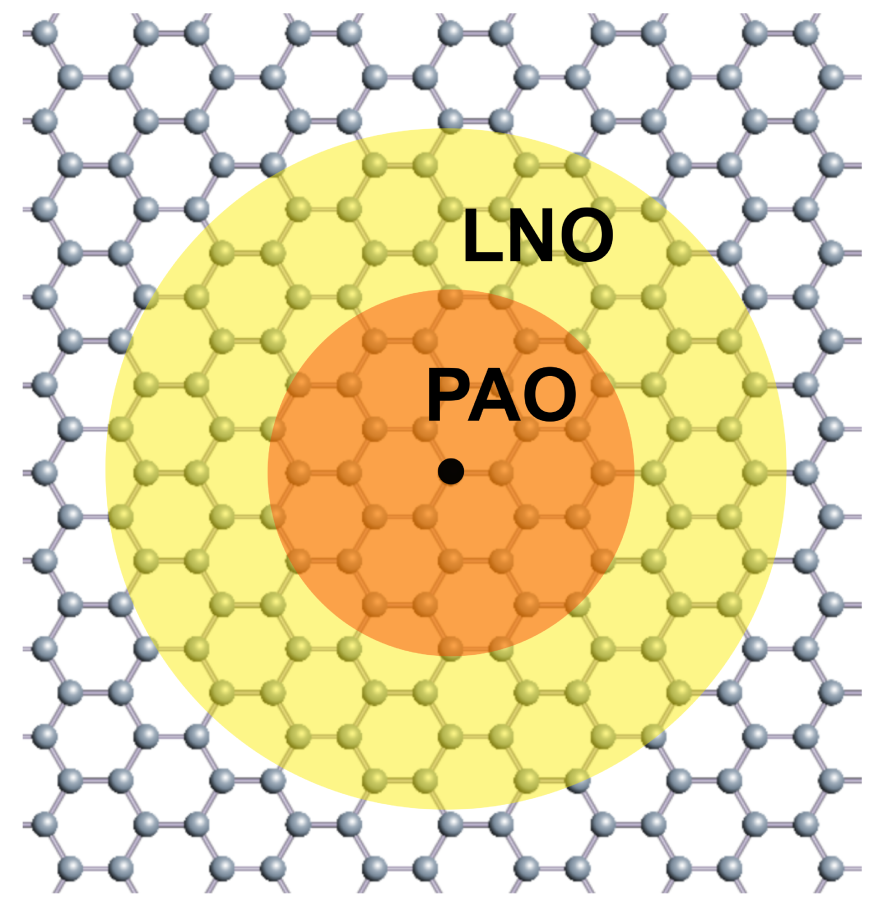
Figure 1: Truncation of a system in the DC method with LNOs. The short range (orange) and long range (yellow) regions are represented by PAOs and LNOs, respectively.
2.2 Generation of LNOs
We present a method of generating LNOs based on a low-rank approximation via a local eigendecomposition of a projection operator. The method might be applicable to any local basis functions, and not limited to the application to the DC method we discuss in the paper. Even in the conventional O() calculations, the LNOs can be easily obtained by a non-iterative calculation using the density matrix and overlap matrix elements. Since a smaller number of LNOs well reproduce dispersion of occupied bands, they can be an alternative basis set for a compact representation for the Hamiltonian and overlap matrices. Though in this subsection we present a method of calculating LNOs in a general form starting from Bloch functions to clarify a mathematical basis of LNOs, it should be clearly noticed in this place that the density matrix is directly calculated in the DC-LNO method without calculating the Bloch functions. The general formulation presented here provides a theoretical basis of three step algorithm which will be discussed in the end of the subsection.
Under the Born-von Karman boundary condition we expand a Kohn-Sham (KS) orbital , indexed with a k-vector in the first Brillouin zone and band index , using PAOs [33, 34], being a real function, as
| (1) |
where , , and are a lattice vector, the number of cells in the boundary condition, and linear combination of pseudo-atomic orbital (LCPAO) coefficients, respectively. It is also noted that and , where and are atomic and orbital indices, respectively, and is the position of atom . We assume that PAO functions are allocated to atom . Throughout the paper we do not consider the spin dependency on the formulation for sake of simplicity, but the generalization is straightforward. By considering overlap matrix elements , one can introduce two alternative localized orbitals:
| (2) | |||||
| (3) |
where and are calculated from an overlap matrix for a supercell consisting of primitive cells in the Born-von Karman boundary condition. Hereafter, and will be referred to as Löwdin [42] and dual orbitals [33], respectively. It is noted that we have the following relations:
| (4) | |||||
| (5) |
and that the identity operator can be expressed in Bloch functions , Löwdin orbitals , or PAOs and dual orbitals as
| (6) | |||||
We now define a projection operator for the occupied space by
| (7) |
where and are the Fermi-Dirac function and an eigenvalue of the KS equation, respectively. By using the second line of Eq. (6), one obtains an alternative expression of the projection operator as
| (8) |
with
where , and is a column vector whose elements are LCPAO coefficients . As well, one can derive another expression of the projection operator by applying the third line of Eq. (6) to Eq. (7) as
| (10) |
with
It is noted that is related to by the following relation:
| (12) |
Remembering that the number of electrons in the supercell consisting of primitive cells can be obtained by the trace of , and that we have two alternative expressions Eqs. (8) and (10) for , one has the following expressions for :
| (13) | |||||
where the factor of 2 is due to spin degeneracy. Since each term in the summation over equally contributes to , we have , where . Thus, it is enough to consider instead of for further discussion. By introducing a notation for a subset of orbitals and with
| (14) | |||||
| (15) |
one can write as
| (16) |
where means a partial trace over orbitals associated with an atom in the central cell with , and is defined by
| (17) |
with definition of block elements:
| (18) | |||||
| (19) |
These block elements and are matrices, where and are the number of PAO functions allocated to atoms and , respectively. Therefore, defined by Eq. (17) is a matrix. It should be emphasized that Eq. (16) giving by the sum of the partial trace is an important relation in calculating LNOs, since it shows that a local similarity transformation on an atomic site does not change because of a property of the trace. Noting that is nonsymmetric, we consider a general eigendecomposition of a nonsymmetric matrix for among similarity transformations as
| (20) |
where is a diagonal matrix having eigenvalues of as diagonal elements. Since an eigenvalue of gives the population for the corresponding eigenstate of , one can distinguish LNOs spanning the occupied space from others among all the eigenstates of by monitoring the eigenvalues. To see the idea more clearly, we define an operator by
| (21) |
where is the -th column vector of , and is the -th row vector of . Note that is the dual orbital of , and . It is easy to confirm that and in a matrix form can be obtained by representing with and , and with and , respectively. Thus, we have . If the eigenvalue is nearly zero, the contribution of the corresponding eigenstate is negligible in the summation of Eq. (21). Therefore, can be approximated by excluding eigenstates whose eigenvalues are less than a threshold value that we will discuss later on. The treatment can be regarded as a low-rank approximation [43]. Then, using Eqs. (16) and (21) we can approximate the projection operator defined by Eq. (7) as
| (22) |
where terms satisfying a condition are taken into account in the summation over . If all the terms are included, Eq. (22) becomes equivalent to Eq. (7). We now define our LNOs by whose eigenvalues are larger than or equal to the threshold value . By comparing Eq. (20) with Eq. (16), one has . Thus, LNOs are defined by , and it should be noted that are the corresponding dual orbitals. The approximate formula Eq. (22) for implies that a set of orbitals , LNOs, well spans the occupied space, while the number of orbitals is reduced compared to the original PAOs. It is worth noting that LNOs can be independently calculated for each atom by a non-iterative calculation via Eqs. (17) and (20). The fact makes the method of generating LNOs very efficient, and also guarantees that the resultant LNOs associated with an atom are expressed by a linear combination of PAOs allocated to only the atom [44].
The computational procedure to generate LNOs is summarized as follows: (i) Calculation of . For each atom the matrix is calculated by Eq. (17), where the summation over is limited within a finite range because of the locality of PAOs in real space. (ii) Diagonalization of . Since the matrix is nonsymmetric, the diagonalization in Eq. (20) is performed by a generalized eigenvalue solver for a nonsymmetric matrix such as DGEEV in LAPACK [48]. (iii) Selection of . Eigenvectors whose eigenvalues are larger than or equal to the threshold value are selected as LNOs. Only the overlap and density matrices are required to calculate LNOs through the steps (i)-(iii) above. Therefore, either conventional O() methods or O() methods can be employed as eigenvalue solver as long as they generate the density matrix. As for LNOs other than those in the central cell with , it is apparent from the derivation that one can obtain by parallel translation of with the lattice vector . The method can also be extended to choose another energy window. In the projection operator defined by Eq. (7), the Fermi-Dirac function is introduced to choose the occupied space. However, one can choose a proper energy window in the definition of the projection operator depending on what we discuss, which enables us to focus on specific bands such as localized -bands near the Fermi level. In this sense, LNOs can be utilized like Wannier functions (WFs) [49, 50], while WFs are obtained through a unitary transformation of Bloch functions rather than the low-rank approximation, and they are orthonormal each other unlike LNOs. It is also worth pointing out that our method shares the basic idea based on the projection with other methods such as the quasiatomic orbitals scheme [51, 52, 53], a projection method [54], and a method via selected columns of the density matrix [55, 56].
It might be possible for the method we present in the paper to be applied for other localized basis functions such as finite element methods [57, 58] and finite difference methods [59, 60, 61]. In those cases one may introduce spatial partitioning methods such as Voronoi tessellation to decompose basis functions rather than focusing on basis functions on a single grid. A similar procedure can be applied for a set of partitioned basis functions.
2.3 DC method with LNOs
Here we consider an extension of the DC method [31, 32] using LNOs discussed in the previous subsection. Our theoretical basis to formulate the O() DC method is that the total energy and atomic forces in the KS framework can be calculated by using electron density , density matrix , and energy density matrix defined by
| (23) | |||||
| (24) |
and
| (25) |
where is the Green function defined by with the overlap matrix and KS matrix , and the factor of 2 in Eq. (23) is due to spin degeneracy. It is remarked that forces on atoms in the DC method are not calculated variationally, but evaluated by using the formula derived by assuming that numerically exact KS wave functions are available as discussed in Ref. [34]. The DC method calculates the Green function approximately by introducing the truncation scheme as shown in Fig. 1. The KS matrix of the truncated cluster for atom are constructed using PAOs and LNOs as follows:
| (26) |
where the top left and bottom right blocks correspond to the short range (orange) region represented by PAOs, and the long range (yellow) region represented by LNOs, respectively, as shown in Fig. 1. The top right and the bottom left block consist of the hopping matrix elements bridging the two regions, and they are represented by both PAOs and LNOs. As well, the same structure is found for the overlap matrix. Noting that the computational bottleneck is mainly governed by the eigenvalue problem for the truncated clusters, and that the matrix size can be reduced by introducing LNOs compared to the conventional DC method, one can expect a considerable reduction of the computational cost as the size of the long range region increases. The idea of reducing the matrix dimension by introducing an effective representation of Hamiltonian is similar to that in the O() Krylov subspace method [34] and the absolutely localized molecular orbitals (ALMO) method [23]. By solving the eigenvalue problem for the truncated cluster of atom , we calculate matrix elements associated with the atom for the Green function as [62]
| (27) |
Matrix elements and associated with the atom can be analytically calculated by inserting Eq. (27) into Eqs. (24) and (25), respectively. We only have to calculate and only if is non zero, since the other elements do not contribute to the total energy and forces on atoms in case of semi-local functionals such as local density approximations (LDA) [63, 64] and generalized gradient approximations (GGA) [65]. Then, in Eq. (23) is easily computed from . By applying the procedure for all the atoms in a system, all the necessary information to calculate the total energy and forces on atoms are obtained.
The overall procedure of the DC method with LNOs is summarized as follows: (i) Calculation of LNOs. LNOs are calculated by Eq. (20) for all atoms in the central cell with . At every SCF step LNOs are updated, leading to self-consistent determination of LNOs. (ii) Construction of and . For each atom the KS and overlap matrices for a truncated cluster associated with the atom are constructed by Eq. (26). (iii) Diagonalization of by making use of a parallel eigenvalue solver. (iv) Finding a common chemical potential to conserve the total number of electrons in the system using Eq. (27), as discussed in Ref. [34] in detail. (v) Calculation of density matrix and energy density matrix using Eqs. (24), (25), and (27). (vi) Calculation of electron density using Eq. (23).
3 IMPLEMENTATIONS
We have implemented the DC-LNO method into the OpenMX DFT software package [66] which is based on norm-conserving pseudopotentials (PPs) [67, 68] and optimized pseudo-atomic orbitals (PAOs) [40, 41] as basis set. All the benchmark calculations were performed with a computational condition of a production level. The basis functions used are C6.0-s2p2d1, Si7.0-s2p2d1, Ti7.0-s2p2d1, O6.0-s2p2d1, Li8.0-s3p2, Al7.0-s2p2d1, and Fe5.5-s3p2d2 for carbon, silicon, titanium, oxygen, lithium, aluminum, and iron, respectively, where in the abbreviation of basis functions such as C6.0-s2p2d1, C stands for the atomic symbol, 6.0 the cutoff radius (Bohr) in the generation by the confinement scheme, and s2p2d1 means the employment of two, two, and one optimized radial functions for the -, -, and -orbitals, respectively. The radial functions were optimized by a variational optimization method [40]. These basis functions we used can be regarded as double zeta plus polarization basis sets if we follow the terminology of Gaussian basis functions. As valence electrons in the PPs we included and , and , , , , and , and , , , and , and , and , , , and states for carbon, silicon, titanium, oxygen, lithium, aluminum, and iron, respectively. All the PPs and PAOs we used in the study were taken from the database (2013) in the OpenMX website [66], which were benchmarked by the delta gauge method [69]. Real space grid techniques are used for the numerical integrations and the solution of the Poisson equation using FFT with the energy cutoff of 300 Ryd [70]. We used a generalized gradient approximation (GGA) proposed by Perdew, Burke, and Ernzerhof to the exchange-correlation functional [65]. An electronic temperature of 300 K is used to count the number of electrons by the Fermi-Dirac function for all the systems we considered.
The short and long range regions depicted in Fig. 1 are determined as follows: (i) We first pick up atoms in a sphere with a given cutoff radius . (ii) Among the atoms selected by the step (i) we distinguish the first neighboring atoms (FNAs) having non-zero overlap with the central atom in terms of basis functions, and remaining atoms other than FNAs are called the second neighboring atoms (SNAs), where the number of FNAs and SNAs are and , respectively. (iii) The short range region is determined by adjusting a cutoff radius so that the number of atoms in a sphere with a radius of can be as close as possible to , where the parameter can vary from 0 to 1, and we will discuss the choice of later on. (iv) The long range region consists of remaining atoms other than atoms selected by the step (iii). If we assign FNAs to atoms in the short range region, the total energy does not converge to the numerically exact one calculated by the conventional diagonalization method even if the cutoff radius increases systematically. This is because the error with the low-rank approximation by Eq. (22) keeps increasing as the cutoff radius increases. To avoid the situation, we add a buffer region consisting of about atoms as described by the step (iii) above, which guarantees the convergence of the total energy and other quantities as a function of the cutoff radius . Throughout the study, we used of for all the systems by taking the accuracy into account more than the efficiency, and did not adjust the parameter, while a smaller value, which well balances both the accuracy and efficiency, can be employed for some systems.
The way of parallelization for the DC-LNO method on parallel computers will be discussed together with its benchmark calculations later on.
4 NUMERICAL RESULTS
4.1 Band dispersions by LNOs
In order to investigate to what extent LNOs can span occupied spaces, we compare band dispersions
of gapped and metallic systems calculated with PAOs and LNOs.
Figure 2(a) and (b) show
band dispersions of diamond and silicon calculated by a conventional O() diagonalization method
with PAOs and LNOs. For both the cases the SCF calculations were performed by using PAOs.
For the case of LNOs the band dispersions were calculated with the LNOs after the SCF calculations
with PAOs. The number of LNOs per atom is 4 for both carbon and silicon atoms.
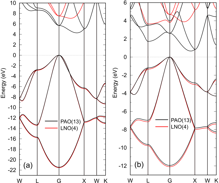
Figure 2: Band dispersions of (a) diamond and (b) silicon in the diamond structure with experimental lattice constants
(3.567 and 5.430 Å) calculated by PAOs (black) and LNOs (red).
A conventional O() method was used for the diagonalization, where
the number of k-points for the Brillouin zone sampling is for both the cases.
In the case of LNOs, the SCF calculations were performed by using PAOs, and after determining the SC
electron density, LNOs were used to calculate the band dispersion. The numbers of PAOs and LNOs
per atom are shown in the parenthesis.
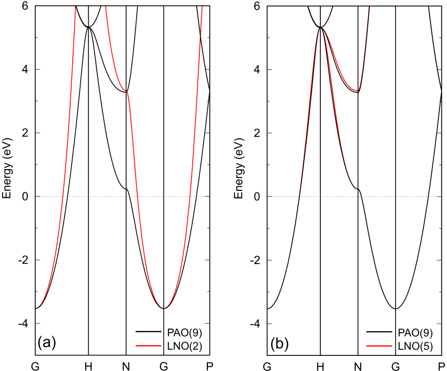
Figure 3: Band dispersions of BCC lithium with an experimental lattice constant of 3.491 Å calculated by PAOs (black) and (a) two and (b) five LNOs (red). The number of k-points for the Brillouin zone sampling is . The other details are the same as in the caption of Fig. 2.
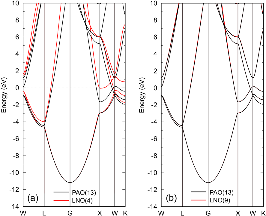
Figure 4: Band dispersions of FCC aluminum with an experimental lattice constant of 4.050 Å calculated by PAOs (black) and (a) four and (b) nine LNOs (red). The number of k-points for the Brillouin zone sampling is . The other details are the same as in the caption of Fig. 2.
| Diamond | Si | Li | Al | |
|---|---|---|---|---|
| 0.514 | 0.639 | 0.999 | 0.551 | |
| 0.483 | 0.430 | 0.277 | 0.253 | |
| 0.483 | 0.430 | 0.075 | 0.253 | |
| 0.483 | 0.430 | 0.075 | 0.253 | |
| 0.012 | 0.018 | 0.074 | 0.049 | |
| 0.012 | 0.018 | 0.001 | 0.049 | |
| 0.012 | 0.018 | 0.001 | 0.049 | |
| 0.011 | 0.012 | 0.001 | 0.033 | |
| 0.011 | 0.012 | -0.002 | 0.033 | |
| -0.001 | 0.002 | - | -0.002 | |
| -0.001 | 0.002 | - | -0.002 | |
| -0.001 | 0.002 | - | -0.002 | |
| -0.018 | -0.011 | - | -0.015 |
4.2 Total energies by DC-LNO
As a first step of validation of the DC-LNO method with respect to computational accuracy and efficiency, we show in Fig. 5 the absolute error in the total energy of gapped and metallic systems calculated by the DC and the DC-LNO methods, where the reference energies were calculated by the conventional O() method with dense k-points for the Brillouin zone sampling as given in the caption of Figs. 2-4. For all the cases the threshold value in Eq. (22) was set to be 0.1 which gives us the minimal LNOs corresponding to orbitals of valence electrons. In the gapped systems, diamond, silicon, and rutile TiO, the absolute error decreases almost exponentially as the number of atoms in a truncated cluster increases. The overall behaviors of the error between the DC and DC-LNO methods are similar to each other, while the error by the DC-LNO method is accidentally much smaller than that by the DC method in the case of large truncated clusters of diamond. As well as the gapped systems the absolute error for metals calculated by the DC-LNO method decreases as increasing the number of atoms in a truncated cluster in a similar way to the DC method. The relatively large oscillating behavior observed in the metals might be related to long range characteristics of the off-diagonal Green functions as discussed in the Appendix. For all the cases including metals it is found that a truncated cluster including about 300 atoms is required to attain the millihartree accuracy corresponding to the error less than a few millihartree/atom in the total energy. From the comparison between the DC and DC-LNO methods, we see that the computational accuracy does not degrade largely even if basis functions for atoms in the long range region are approximated by LNOs, and that thereby the computational accuracy can be controlled mainly by the size of truncated cluster just like for the DC method. Since controlling only the single parameter allows us to balance the computational accuracy and efficiency, it is expected that the feature makes the DC-LNO method easy to use for a wide variety of applications.
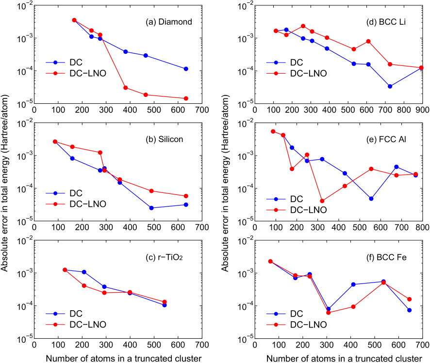
Figure 5: Absolute error in the total energy (Hatree/atom) for (a) diamond, (b) silicon in the diamond structure, (c) rutile TiO, (d) BCC lithium, (e) FCC aluminum, and (f) BCC iron as a function of the number of atoms in a truncated cluster calculated by the DC and DC-LNO methods. The experimental lattice constants were used for all the cases.
4.3 Computational time
Since the total number of basis functions to represent the Hamiltonian of the truncated cluster is reduced by introducing LNOs while keeping the accuracy, it is expected that the computational time can be substantially reduced. In the whole procedure of the DC-LNO method the calculation of LNOs and construction of Hamiltonian and overlap matrices occupy a small fraction of the whole computational time, typically less than , and thereby the computational time is mainly governed by solving of the eigenvalue problem for each atom . Noting that the computational time to solve the eigenvalue problem scales as the third power of the dimension of the matrices, the ratio of computational time between the DC-LNO and DC methods for elemental systems might be estimated by
| (28) |
where and are the number of PAOs and LNOs associated with each atom, respectively, and is a factor, which is fixed to in this study, to control the size of the buffer region as discussed in the section ’IMPLEMENTATIONS’. For example, if the cutoff radius is set to be Å in the diamond structure with the experimental lattice constant of 3.567 Å, and are found to be 167 and 298, and the resultant number of atoms in the short (long) range region becomes 275 (190). Then, can be estimated to be 0.37 in the case that the number of PAOs and LNOs per atom is 13 and 4, which implies that the computational time of the DC-LNO method becomes about one third of that calculated by the DC method. Figure 6 shows actual timing results of the DC and DC-LNO methods for (a) diamond and (b) BCC lithium. We see that the actual for the diamond case is 0.40 in the case that the number of atoms is 465 (=167+298) as shown in Fig. 6(a), which is well compared to the estimated value of 0.37. As indicated by Eq. (28) and in Figs. 6(a) and (b), it is concluded that the DC-LNO method becomes much faster than the DC method as the size of the truncated cluster increases.
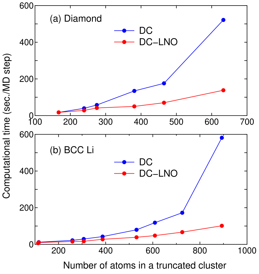
Figure 6: Comparison of computational time of the diagonalization part per molecular dynamics (MD) step between the DC and DC-LNO methods for (a) diamond and (b) BCC lithium. Both the calculations were performed for the primitive cell using 14 MPI processes per atom on Intel Xeon CPUs E5-2690v4 @ 2.60 GHz.
In Fig. 7 we further show timing results of the DC-LNO method as a function of the number of atoms in the unit cell of Si crystal. It is confirmed from the linear increase of the computational time that the DC-LNO method is a linear scaling approach in practice. As a comparison the computational time is also shown for the conventional diagonalization method [73]. The crossing point between the two methods in the computational time is located around 100 atoms when 1280 CPU cores is used. Over 100 atoms the DC-LNO method is much faster than the conventional diagonalization method. The reason why the crossing point is located at such a small number of atoms is partly due to a better parallel efficiency of the DC-LNO method as discussed in the next subsection.
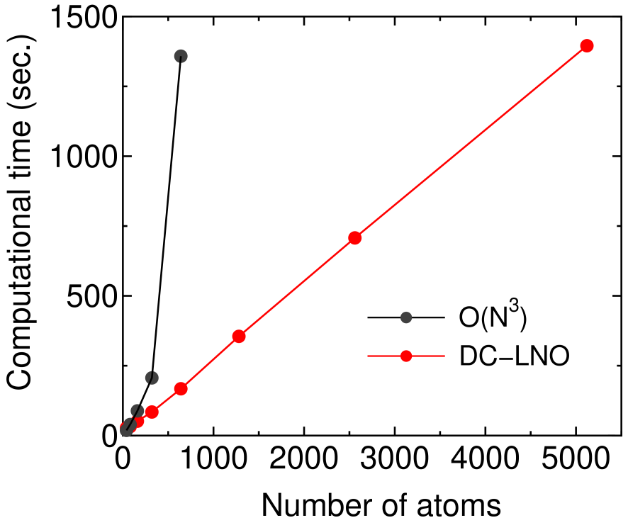
Figure 7: Computational time (sec.) of the diagonalization part per 10 SCF steps for Si in the diamond structure. In the DC-LNO method the cutoff radius of Å was used, resulting in the truncated cluster containing 293 atoms. In the O() method the k-grids of were used for the Brillouin zone sampling in all the cases. All the calculations were performed using 1280 MPI processes on a cluster machine consisting of Intel Xeon CPUs E5-2680v2 @ 2.80 GHz connected with Infiniband 4X FDR @ 56 Gbps.
4.4 Parallelization
To minimize the computational time on massively parallel computers we introduce a multilevel parallelization using message passing interface (MPI). In our implementation there are three levels for the parallelization, i.e., atom level, spin level, and diagonalization level as explained below: (i) Parallelization in the atom level. If the number of MPI processes is smaller than that of atoms, only the parallelization in the atom level is taken into account. The allocation of atoms to MPI processes is performed by a bisection method which is based on a projection of atoms onto a principal axis calculated from an inertia tensor and a modified binary tree of MPI processes to minimize memory usage and amount of MPI communications [36]. (ii) Parallelization in the spin level. If the number of MPI processes exceeds that of atoms, and the spin polarized calculation is performed, the parallelization in the spin level is introduced on top of the parallelization in the atom level, where a loop for the spin index is further parallelized. (iii) Parallelization in the diagonalization level. If the number of MPI processes is larger than the product of the number of atoms and the multiplicity of spin index, corresponding to 1, 2, and 1 for non-spin polarized, spin-polarized, and non-collinear calculations, respectively, a parallelization in the diagonalization level is further taken into account on top of both the parallelizations in the atom and spin levels. The parallelization in the diagonalization level is made by employing a parallel eigenvalue solver ELPA [73]. It is noted that the parallelization in the diagonalization level requires a considerable amount of MPI communications, while the parallelizations in the atom and spin levels have less MPI communications. So, one would expect a high parallel efficiency in the atom and spin levels, while the parallelization in the diagonalization level might be limited up to several tens of MPI processes. To achieve a better scaling for the parallelization in the diagonalization level, it is important to allocate CPU cores in the same computer node as MPI processes to avoid the inter-node communication as much as possible. We have implemented the multilevel parallelization so that amount of the inter-node communication can be minimized especially for the parallelization in the diagonalization level. In Fig. 8 the speed-up ratio in the MPI parallelization of the DC-LNO method is shown for non-spin polarized calculations of a diamond supercell containing 64 atoms. Since the multiplicity of spin index is 1, we see a nearly ideal behavior up to 64 MPI processes. Beyond 64 MPI processes the parallelization in the diagonalization level is taken into account on top of the parallelization in the atom level. A superlinear speed-up is observed at 128 and 256 MPI processes, which might be due to an effective use of cache by the reduction of memory usage, and a good scaling is achieved up to 1280 MPI processes at which the parallel efficiency is calculated to be 70% using the elapsed time at 1 MPI process as reference. Since each computer node has 20 CPU cores in this case, it would be reasonable to observe the good scaling up to 1280 (=6420) MPI processes. Thus, we see that the multilevel parallelization is very effective to minimize the computational time in accordance with a recent development of massively parallel computers.
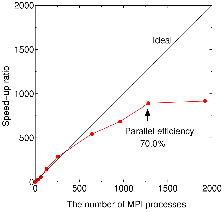
Figure 8: Speed-up ratio in the MPI parallelization of the DC-LNO method for a diamond supercell containing 64 atoms, where the cutoff radius of Å was used, leading to the numbers of atoms of 239 and 142 in the short and long range regions, and the dimension of matrices of 3675 for the truncated cluster problem. The calculations were performed using the same cluster machine as for Fig. 7.
4.5 Molecular dynamics simulations
To verify the accuracy of forces on atoms calculated by the DC-LNO method, results of NVE molecular dynamics (MD) simulations are shown in Fig. 9. We see that the sum of the kinetic energy of atomic nuclei (Kinetic) and the internal total energy (), being a conserved quantity, is reasonably conserved as a function of time, and the fluctuation is about one tenth of the kinetic energy or the internal total energy. It should be noted that the approximate conservation of the sum is achieved for not only Si being a semi-conductor, but also Al being a metal. Thus, it can be concluded that the accuracy of forces on atoms calculated by the DC-LNO method is sufficient for practical purposes, while it was remarked in the Sec. II that the forces on atoms in the DC-LNO method are not calculated variationally. The sufficient accuracy of the calculated forces is achieved by the use of large cutoff radii in constructing the truncation clusters, which is realized by both the introduction of LNOs and the massive parallelization with the multilevel parallelism.
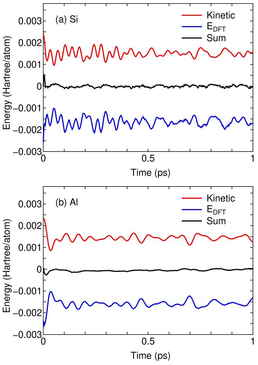
Figure 9: The kinetic energy of atomic nuclei (Kinetic), the internal total energy (), and the sum of them as a function of time in NVE molecular dynamics simulations by the DC-LNO method for (a) Si and (b) Al, where the time step of 2 fs was used, and random velocities corresponding to 400 K were given for atomic nuclei at the first MD step. The simulation cells with experimental lattice constants for Si and Al contain 64 and 108 atoms, respectively. For the DC-LNO method the cutoff radii of 11.3 and 10.1 Å were used for Si and Al, respectively, resulting in the truncated cluster containing 293 and 249 atoms in the ideal bulk structure. Each energy curve was shifted by adding a constant.
To further demonstrate the applicability of the DC-LNO method for MD simulations, we show radial distribution functions (RDFs) in liquid phases of silicon, aluminum, lithium, and SiO in Fig. 10. Since the electronic structures exhibit metallic features in the liquid phases of silicon, aluminum, and lithium, the MD simulations can be considered as a severe benchmark to validate the applicability of the DC-LNO method to metals. The cutoff radii we used correspond to truncated clusters consisting of about 300 atoms in the ideal bulk structures. It turns out that in all the cases the DC-LNO method reproduces well the results by the conventional diagonalization method, and that the obtained RDFs are well compared to other computational results [75, 76, 77, 78]. The considerable agreement between the DC-LNO and conventional methods strongly implies that a sufficient accuracy in reproducing at least RDF for MD simulations can be attainable with a cutoff radius resulting in truncated clusters consisting of about 300 atoms for not only insulators but also metals. Thus, adjusting the cutoff radius so that the number of atoms in a truncated cluster can be 300 atoms would be a compromise to balance the computational accuracy and efficiency, while the difference between the DC and DC-LNO methods in terms of the computational efficiency may not be significant for truncated clusters of this size. It is crucial to minimize the elapsed time for realization of long time MD simulations. With the computational condition the elapsed time per SCF step for silicon is 1.5 (sec.) on average using 1280 MPI processes on the same machine used for the calculations shown in Fig. 8.
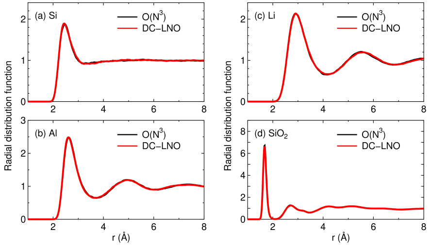
Figure 10: Total radial distribution function (RDF) of (a) silicon at 3500 K, (b) aluminum at 2500 K, (c) lithium at 800 K, and (d) SiO at 3000 K, calculated by the conventional diagonalization and the DC-LNO methods. The MD simulations were performed for cubic supercells containing 64, 108, 128 and 192 atoms with a fixed lattice constant of 10.86, 12.15, 14.04, 14.25 Å for silicon, aluminum, lithium, and SiO, respectively, for 10 ps with the time step of 2 fs. The temperature was controlled by a velocity scaling scheme by Woodkock [74]. The coordinates for the first 1 ps were excluded to calculate RDF. In the DC-LNO method the cutoff radii of 11.3, 10.1, 12.5, and 11.0 were used for silicon, aluminum, lithium, and SiO, respectively, resulting in truncated clusters consisting of 293, 249, 339, and 344 (on average) atoms in the ideal bulk structures. In the conventional diagonalization method, k-points of , , , and were used for the Brillouin zone sampling in silicon, aluminum, lithium, and SiO, respectively,
5 CONCLUSIONS
We have presented an efficient O() method based on the DC approach and a coarse graining of basis functions by localized single-particle natural orbitals (LNOs) for large-scale DFT calculations. A straightforward way to attain sufficient accuracy in the DC method is to employ a relatively large cutoff radius for the truncation of a system, which is the most fundamental parameter in most of O() methods to control the computational accuracy and efficiency. We have adopted the rather brute force approach, and attempted to decrease the computational cost by introducing LNOs as basis functions in the long range region of the truncated cluster, and to minimize the elapsed time in the computation with the help of a multilevel parallelization. The method of generating LNOs is based on a low-rank approximation to the projection operator for the occupied space by a local eigendecomposition at each atomic site, and the band structure calculations with PAOs and LNOs clearly show that the resultant LNOs span well the occupied space of not only gapped systems but also metals. It is also worth mentioning that the computational cost of generating LNOs is almost negligible thank to the independent calculation at each atomic site. By replacing PAOs with LNOs in the long range region of the truncated cluster in the DC method, the computational cost of the DC method can be reduced without largely sacrificing the accuracy. Nothing that the DC-LNO method holds the simple algorithm of the original DC method suited to the parallel calculation, we have implemented a multilevel parallelization using MPI by taking account of the atom level, spin level, and diagonalization level. It was demonstrated that the speed-up of the DC-LNO method by the multilevel parallelization can be expected up to a specific number of MPI processes which corresponds to the product of the number of atoms, the multiplicity of spin index, and the number of CPU cores in a single computer node. For example, if a spin-polarized calculation is performed for a system consisting of 1000 atoms on a parallel computer with 20 CPU cores per node, a high parallel efficiency might be expected up to 40000 MPI processes. As a validation of the applicability of the DC-LNO method, we have performed MD simulations for liquid phases of an insulator, semi-conductor, and metals, and confirmed that the RDFs calculated by the DC-LNOs are in good agreement with those by the conventional diagonalization method, which may lead to its various applications to structural determinations of amorphous and liquid structures of complicated materials [79, 80, 81, 82, 83]. Considering the simplicity and robustness of the algorithm, we conclude that the DC-LNO method is an efficient and accurate approach to large-scale DFT calculations for a wide variety of materials including metals.
ACKNOWLEDGMENT
This work was supported by Priority Issue (Creation of new functional devices and high-performance materials to support next-generation industries) to be tackled by using Post ’K’ Computer, MEXT, Japan. Part of the computation in the study was performed using the computational facility of the Japan Advanced Institute of Science and Technology.
Appendix A: Asymptotic behaviors of the off-diagonal Green functions
As an example we show asymptotic behaviors of the off-diagonal Green functions for an one-dimensional (1D) tight-binding (TB) model with a single -orbital on each site, and relate the asymptotic behaviors to electronic structures in gapped and metallic systems. The analysis interprets evidently the oscillating behavior of the error in the total energy of the metallic systems as shown in Fig. 5, and the rapid convergence in a high electronic temperature [33, 24].
Let us consider an orthogonal chain model with the nearest neighbor interaction and the on-site energy as defined by
| (29) |
where is assumed to be positive. By tri-diagonalizing the Hamiltonian with a Lanczos algorithm starting from a site (), and calculating the diagonal Green function via a continued fraction using the recursion method [84, 85], one obtains a well known result for the diagonal Green function as follows:
| (30) |
The off-diagonal Green functions can be obtained by using a recurrence relation [86] derived from , where and are the Green function and Hamiltonian matrices represented by the Lanczos vectors, and by performing a back unitary transformation as
| (31) | |||||
| (32) | |||||
| (33) | |||||
| (34) |
where and is the off-diagonal element of Green function between the sites and . It turns out that the off-diagonal Green functions can be expressed by and . To see asymptotic behaviors of the off-diagonal Green functions, by employing the following formula [87]:
| (35) |
with the radius of convergence , we Taylor exand at as
| (36) | |||||
where the convergence is guaranteed for . By inserting Eq. (36) into Eqs. (31)-(34), and taking the leading terms, we obtain the following relation:
| (37) |
Thus, we see that approaches to zero asymptotically for as . On the other hand the Green functions at corresponding to are given by
| (38) | |||||
| (39) |
where . It is found that at exhibits an oscillating behavior as a function of , and never decays.
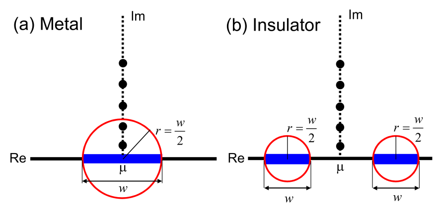
Figure A.1: Relation between the position of Matsubara poles (black filled circels), the spectrum range on the real axis (blue filled rectangles), and the convergent region of the off-diagonal Green functions whose boundaries are shown by red circles in the complex plane for (a) metal and (b) insulator. In the simple TB model the band width is given by , and the off-diagonal Green functions decays asymptotically as increases in the exterior region of the red circles.
We now relate the asymptotic behaviors of Green functions to the calculation of density matrix which is defined by Eq. (24). Introducing the Matsubara expansion of the Fermi-Dirac function, and changing the integration path with the Cauchy theorem, one has [88]
| (40) |
where are Matsubara poles located at with a chemical potential of and . The expression allows us to figure out a relation between the Matsubara poles, where the Green functions are evaluated, and the convergent region of the off-diagonal Green functions as illustrated in Fig. A.1. Remembering that in the simple TB model the band width is given by , and assuming that the single band is half filled in the metallic case, we may have Matsubara poles in the red circle which is the non-convergent region of the off-diagonal Green functions as shown in Fig. A.1(a). Since the off-diagonal Green functions evaluated at the Matsubara poles in the red circle do not simply decay in real space as increases, the truncation scheme commonly adopted in most of O() methods should suffer from the long range characteristics of the off-diagonal Green functions, while the effect can appear in a different way depending on underlying principles of each O() method. In the DC-LNO method the truncated eigenvalue problem is solved for each atom , and the integrations of Eqs. (24) and (25) can be easily performed on the real axis since we have the approximate spectrum representation of Eq. (27). The way of evaluating the density matrix is numerically equivalent to the computational method via a generalized formula of Eq. (40) to the non-orthogonal basis set, where the Green functions for the truncated problem are computed at each Matsubara pole by the inverse calculation, since the Green function computed through the spectrum representation is exactly the same as one computed by the inverse calculation. Therefore, the oscillating behavior of error in the total energy calculation observed in Figs. 5(d), (e), and (f) should be attributed to the long range characteristics of the off-diagonal Green functions. It can also be understood that the use of a higher electronic temperature suppresses the deficiency since all the Matsubara poles can be placed in the exterior region of the red circles beyond a critical temperature [33, 24]. On the other hand we model an insulator by considering two bands as shown in Fig. 1(b), where each of them is expressed by the 1D TB model and the bands are separated by a finite gap. Unlike the metallic case, all the Matsubara poles are located in the exterior region of the red circles. The feature guarantees that decays as increases since all the Green functions in the summation of Eq. (40) decay as increases, theoretically justifying that the truncation scheme is valid for gapped systems, although our benchmark calculations imply that the use of a large cutoff radius diminishes the effect of the long range characteristics of the off-diagonal Green functions even to metals at least for the calculations of density matrix and energy density matrix in a practical sense.
References
- [1] P. Hohenberg and W. Kohn, Phys. Rev. 136, B864 (1964).
- [2] W. Kohn and L. J. Sham, Phys. Rev. 140, A1133 (1965).
- [3] F. Neese, Coordin. Chem.y Rev. 253, 526 (2009).
- [4] R.O. Jones, Rev. Mod. Phys. 87, 897 (2015).
- [5] D.J. Cole and N.D.M. Hine, J. Phys.: Condens. Matter 28, 393001 (2016).
- [6] A. Jain, Y. Shin, and K.A. Persson, Nature Rev. Mat. 1, 15004 (2016).
- [7] H. Sawada, S. Taniguchi, K. Kawakami, and T. Ozaki, Modelling Simul. Mater. Sci. Eng. 21, 045012 (2013).
- [8] H. Sawada, S. Taniguchi, K. Kawakami, and T. Ozaki, Metals 7, 277 (2017).
- [9] M. Wakeda, T. Tsuru, M. Kohyama, T. Ozaki, H. Sawada, M. Itakura, and S. Ogata, Acta Materialia 131, 445 (2017).
- [10] L. Lin, J. Lu, L. Ying, R. Car, and W. E, Commun. Math. Sci. 7, 755 (2009).
- [11] T. Ozaki, Phys. Rev. B 82, 075131 (2010).
- [12] S. Goedecker, Rev. Mod. Phys. 71, 1085 (1999).
- [13] D.R. Bowler and T. Miyazaki, Rep. Prog. Phys. 75, 036503 (2012).
- [14] J. Aarons, M. Sarwar, D. Thompsett, and C.-K. Skylaris, J. Chem. Phys. 145, 220901 (2016).
- [15] J.M. Soler, E. Artacho, J.D. Gale, A. García, J. Junquera, P. Ordejón, and D. Sánchez-Portal, J. Phys.: Condens. Matter 14, 2745 (2002).
- [16] M.J. Gillan, D.R. Bowler, A.S. Torralba and T. Miyazaki, Comp. Phys. Commun. 177, 14 (2007).
- [17] C.-K. Skylaris, P. D. Haynes, A. A. Mostofi, and M. C. Payne, J. Chem. Phys. 122, 084119 (2005).
- [18] E. Tsuchida, J. Phys. Soc. Japan 76, 034708 (2007).
- [19] F. Shimojo, R.K. Kalia, A. Nakano, and P. Vashishta, Phys. Rev. B 77 085103 (2008).
- [20] S. Mohr, L.E. Ratcliff, L. Genovese, D. Caliste, P. Boulanger, S. Goedecker, and T. Deutsch, Phys. Chem. Chem. Phys. 17, 31360 (2015).
- [21] J. VandeVondele, M. Krack, F. Mohamed, M. Parrinello, T. Chassaing, and J. Hutter, Comput. Phys. Commun. 167, 103 (2005).
- [22] J. VandeVondele, U. Bors̆tnik, and J. Hutter, J. Chem. Theory Comput. 8, 3565 (2012).
- [23] R.Z. Khaliullin, J. VandeVondele, and J. Hutter, J. Chem. Theory Comput. 10, 4421 (2013).
- [24] F.R. Krajewski and M. Parrinello, Phys. Rev. 71, 233105 (2005).
- [25] G.S. Ho, V.L. Lignéresa, and E.A. Carter, Comput. Phys. Commun. 179, 839 (2008).
- [26] J.E. Inglesfield, J. Phys. C: Solid State Phys. 14, 3795 (1981).
- [27] Y. Wang, G.M. Stocks, W.A. Shelton, D.M.C. Nicholson, Z. Szotek, and W.M. Temmerman, Phys. Rev. Lett. 75, 2867 (1995).
- [28] R. Zeller, P. H. Dederichs, B. Újfalussy, L. Szunyogh, and P. Weinberger, Phys. Rev. B 52, 8807 (1995).
- [29] R. Zeller, J. Phys.: Condens. Matter 20, 294215 (2008).
- [30] L. Lin and L. Zepeda-Nez, arXiv:1807.08859.
- [31] W. Yang, Phys. Rev. Lett. 66, 1438 (1991).
- [32] W. Yang and T. Lee, J. Chem. Phys. 163, 5674 (1995).
- [33] T. Ozaki, Phys. Rev. B 64, 195126 (2001).
- [34] T. Ozaki, Phys. Rev. B 74, 245101 (2006).
- [35] F. Shimojo, R.K. Kalia, A. Nakano, and P. Vashishta, Comput. Phys. Commun. 167, 151 (2005).
- [36] T.V.T. Duy and T. Ozaki, Comput. Phys. Commun. 185, 777 (2014).
- [37] T. Ohwaki, M. Otani, T. Ikeshoji, and T. Ozaki, J. Chem. Phys. 136, 134101 (2012).
- [38] T. Ohwaki, M. Otani, and T. Ozaki, J. Chem. Phys. 140, 244105 (2014).
- [39] T. Ohwaki, T. Ozaki, Y. Okuno, T. Ikeshoji, H. Imai, and M. Otani, Phys. Chem. Chem. Phys. 20, 11586 (2018).
- [40] T. Ozaki, Phys. Rev. B. 67, 155108, (2003).
- [41] T. Ozaki and H. Kino, Phys. Rev. B 69, 195113 (2004).
- [42] P.-O. Löwdin, J. Chem. Phys. 18, 365 (1950).
- [43] To perform the low-rank approximation, a Schur decomposition which is a similarity transformation can also be considered. However, an ordered Schur decomposition, which orders diagonal elements of the upper triangular matrix in descending order, is required to extract a subspace for a set of LNOs, and the algorithm has not been available in popular libraries such as LAPACK [48]. Another choice is a singular value decomposition (SVD), which has been widely used for low-rank approximations in many fields. While SVD might work in a similar way, it should be noted that SVD is not a similarity transformation, and the singular values do not correspond to the populations.
- [44] It is worth mentioning that a generalization in the approach is to expand LNOs with multisite PAOs including contributions of the central and neighboring atoms [45, 46, 47]. A study toward this direction will be in a future work.
- [45] M.J. Rayson and P.R. Briddon, Phys. Rev. B 80, 205104 (2009).
- [46] A. Nakata, D.R. Bowler, and T. Miyazaki, J. Chem. Theory Comput. 10, 4813 (2014).
- [47] A. Nakata, D. R. Bowler, and T. Miyazaki, Phys. Chem. Chem. Phys. 17, 31427 (2015).
- [48] E. Anderson, Z. Bai, C. Bischof, L.S. Blackford, J. Demmel, J. Dongarra, J. Du Croz, A. Greenbaum , S. Hammarling , A. McKenney, and D. Sorensen, LAPACK Users’ Guide 3rd edn Philadelphia, PA: Society for Industrial and Applied Mathematics), 1999.
- [49] N. Marzari and D. Vanderbilt, Phys. Rev. B 56, 12847 (1997).
- [50] N. Marzari, A.A. Mostofi, J.R. Yates, I. Souza, and D. Vanderbilt, Rev. Mod. Phys. 84, 1419 (2012).
- [51] W.C. Lu, C.Z. Wang, T.L. Chan, K. Ruedenberg, and K.M. Ho, Phys. Rev. B 70, 041101(R) (2004).
- [52] T.-L. Chan, Y.X. Yao, C.Z. Wang, W.C. Lu, J.Li, X.F. Qian, S. Yip, and K.M. Ho, Phys. Rev. B 76, 205119 (2007).
- [53] X. Qian, J. Li, L. Qi, C.-Z. Wang, T.-L. Chan, Y.-X. Yao, K.-M. Ho, and S. Yip, Phys. Rev. B 78, 245112 (2008).
- [54] S. Goedecker, J. Comput. Phys. 118, 261 (1995).
- [55] D. Anil, L. Lin, and Y. Lexing, J. Chem. Theory Comput. 11, 1463 (2015).
- [56] D. Anil, L. Lin, and Y. Lexing, J. Comput. Phys. 334, 1 (2017).
- [57] E. Tsuchida and M. Tsukada, Phys. Rev. B 54, 7602 (1996).
- [58] J.-L. Fattebert, R.D. Hornung, A.M. Wissink, J. Comput. Phys. 223, 759 (2007).
- [59] J.R. Chelikowsky, N. Troullier, and Y. Saad, Phys. Rev. Lett. 72, 1240 (1994).
- [60] J. Iwata, D. Takahashi, A. Oshiyama, T. Boku, K. Shiraishi, S. Okada, K. Yabana, J. Comput. Phys. 229, 2339 (2010).
- [61] T. Ono and K. Hirose, Phys. Rev. B 72, 085115 (2005).
- [62] Although the matrix elements of the Green function associated with only the central atom in the calculation of each truncated cluster are calculated in our implementation, it is possible to generalize the single central atom to a cluster consisting of several atoms. An optimum size of the central cluster might be adjusted in order to reduce the computational cost as discussed in the Appendix of Ref. [34]. However, symmetries in bulks, as can be confirmed in charge density and Mulliken populations, tend to be violated by introducing the central cluster instead of the single central atom. Therefore, we choose the single central atom rather than the central cluster in order to preserve the symmetrical properties.
- [63] D.M. Ceperley and B.J. Alder, Phys. Rev. Lett. 45, 566(1980).
- [64] J.P. Perdew and A. Zunger, Phys. Rev. B 23, 5048 (1981).
- [65] J.P. Perdew, K. Burke, and M. Ernzerhof, Phys. Rev. Lett. 77, 3865 (1996).
- [66] The code, OpenMX, pseudo-atomic basis functions, and pseudopotentials are available under terms of the GNU-GPL on a web site (http://www.openmx-square.org/).
- [67] I. Morrison, D.M. Bylander, L. Kleinman, Phys. Rev. B 47, 6728 (1993).
- [68] G. Theurich and N.A. Hill, Phys. Rev. B 64, 073106 (2001).
- [69] K. Lejaeghere, G. Bihlmayer, T. Björkman, P. Blaha, S. Blügel, V. Blum, D. Caliste, I.E. Castelli, S.J. Clark, A. Dal Corso, S. de Gironcoli, T. Deutsch, J.K. Dewhurst, I. Di Marco, C. Draxl, M. Dułak, O. Eriksson, J.A. Flores-Livas, K.F. Garrity, L. Genovese, P. Giannozzi, M. Giantomassi, S. Goedecker, X. Gonze, O. Grånäs, E.K. Gross, A. Gulans, F. Gygi, D.R. Hamann, P.J. Hasnip, N.A. Holzwarth, D. Iu̧san, D.B. Jochym, F. Jollet, D. Jones, G. Kresse, K. Koepernik, E. Küçü kbenli, Y.O. Kvashnin, I.L. Locht, S. Lubeck, M. Marsman, N. Marzari, U. Nitzsche, L. Nordströ m, T. Ozaki, L. Paulatto, C.J. Pickard, W. Poelmans, M.I. Probert, K. Refson, M. Richter, G.M. Rignanese, S. Saha, M. Scheffler, M. Schlipf, K. Schwarz, S. Sharma, F. Tavazza, P. Thunströ m, A. Tkatchenko, M. Torrent, D. Vanderbilt, M.J. van Setten, V. Van Speybroeck, J.M. Wills, J.R. Yates, G.X. Zhang, and S. Cottenier, Science 351, aad3000 (2016).
- [70] T. Ozaki and H. Kino, Phys. Rev. B 7̱2, 045121 (2005).
- [71] M.-H. Whangbo and H. Hoffmann, J. Chem. Phys. 68, 5498 (1978).
- [72] J.S. Gómez-Jeria, J. Chil. Chem. Soc. 54, 482 (2009).
- [73] A. Marek, V. Blum, R. Johanni, V. Havu, B. Lang, T. Auckenthaler, A. Heinecke, H.-J. Bungartz, and H. Lederer, J. Phys.: Condens. Matter 26, 213201 (2014).
- [74] L.V. Woodcock, Chem. Phys. Lett. 10, 257 (1971).
- [75] J. Behler and M. Parrinello, Phys. Rev. Lett. 98, 146401 (2007).
- [76] V. Recoules and J.-P. Crocombette, Phys. Rev. B 72, 104202 (2005).
- [77] J.A. Anta and P.A. Madden, J. Phys.: Condens. Matter 11, 6099 (1999).
- [78] M. Kim, K.H. Khoo, J.R. Chelikowsky, Phys. Rev. B 86, 054104 (2012).
- [79] A. Sakuda, K. Ohara, K. Fukuda, K. Nakanishi, T. Kawaguchi, H. Arai, Y. Uchimoto, T. Ohta, E. Matsubara, Z. Ogumi, T. Okumura, H. Kobayashi, H. Kageyama, M. Shikano, H. Sakaebe, and T. Takeuchi, J. Am. Chem. Soc. 139, 8796 (2017).
- [80] A. Sakuda, T. Takeuchi, M. Shikano, K. Ohara, K. Fukuda, Y. Uchimoto, Z. Ogumi, H. Kobayashi, and H. Sakaebe, J. Ceram. Soc. Jpn. 125, 268 (2017).
- [81] N. Ileri and L.E. Fried, Theoretical Chemistry Accounts 133, 1575 (2014).
- [82] L. Koziol, L.E. Fried, and N. Goldman, J. Chem. Theory Comput. 13, 135 (2017).
- [83] Y. Feng, Y. Zhang, G. Du, J. Zhang, M. Liu, and X. Qu, New J. Chem. 42, 13775 (2018).
- [84] R. Haydock, V. Heine, and M.J. Kelly, J. Phys. C 5, 2845 (1972); 8, 2591 (1975).
- [85] R. Haydock, Solid State Phys. 35, 216 (1980).
- [86] T. Ozaki, M. Aoki, and D.G. Pettifor, Phys. Rev. B 61, 7972 (2000).
- [87] “Table of Integrals, Series, and Products”, I.S. Gradshteyn and I.M. Ryzhik, A. Jeffrey (Ed.), and D. Zwillinger (Ed.), Academic Press, Seventh Edition, 2007.
- [88] T. Ozaki, Phys. Rev. B 75 035123 (2007).