Efficient Integration of Green’s functions: Ver. 1.1
The original has been published
in Phys. Rev. B 75, 035123 (2007).
Abstract
An efficient and accurate contour integration method is presented for large-scale electronic structure calculations based on the Green function. By introducing a continued fraction representation of the Fermi-Dirac function derived from a hypergeometric function, the Matsubara summation is generalized with respect to distribution of poles so that the integration of the Green function can converge rapidly. Numerical illustrations, evaluation of the density matrix for a simple model Green function and a total energy calculation for aluminum bulk within density functional theory, clearly show that the method provides remarkable convergence with a small number of poles, indicating that the method can be applied to not only the electronic structure calculations, but also a wide variety of problems.
1 INTRODUCTION
The integration of the Green function associated with the Fermi-Dirac function is one of the most important ingredients for accurate and efficient implementation of electronic structure calculation methods regardless of ab initio or semi-empirical schemes. One can realize that the integration arises in lots of electronic structure calculation methods such as the Korringa-Kohn-Rostoker (KKR) Green function method,[1, 2, 3] Green function based O() methods such as a recursion method,[4, 5] a surface Green function method[6] such as an embedded method,[7] and Green function methods based on a many body perturbation theory such as the GW method.[8, 9] Therefore, it is obvious that a highly accurate and efficient method must be developed for the integration to extend applicability of these electronic structure calculation methods. Since the well-known Matsubara summation [15, 16] is insufficient for this purpose due to the slow convergence, considerable efforts have been devoted for development of efficient integration methods.[10, 11, 12, 13, 14] A way of developing an efficient method beyond the Matsubara summation is to seek another expression for the Fermi-Dirac function. Along this line, an expression is used by Nicholson et al.,[10] and an integral representation is proposed by Goedecker.[11] In this paper I seek a different expression for the Fermi-Dirac function, and present an accurate and efficient method for the integration, based on a continued fraction representation of the Fermi-Dirac function which is derived from a hypergeometric function. Because of a simple distribution of poles in the continued fraction similar to the Matsubara poles, it is anticipated that the proposed method can be easily incorporated into many applications with the same procedure as for the Matsubara summation but with remarkable efficiency. It will be shown that the rapid convergence in the integration can be attributed to an interesting non-uniform distribution of the poles on the imaginary axis, and that even a small number of poles in the contour integration enables us to achieve convergent results with precision of more than ten digits. This paper is organized as follows: In Sec. II the theory of the proposed method is presented with comparison to other methods. In Sec. III in order to illustrate the rapid convergence properties of the proposed method I give two numerical examples: a calculation of the density matrix for a simple model Green function and a total energy calculation of aluminum bulk within a density functional theory. In Sec. IV the theory and applicability of the proposed method are summarized.
2 THEORY
2.1 Continued fraction representation of the Fermi-Dirac function
Let us introduce a continued fraction representation of the Fermi-Dirac function which is derived from a hypergeometric function:
| (1) |
where with , is chemical potential, electronic temperature, and are complex variables. The derivation of Eq. (1) is given in the Appendix A. Figure 1 shows the approximate Fermi-Dirac function terminated at 60 levels of the continued fraction given by Eq. (1) as a function of together with the exact Fermi-Dirac function, with , and the Matsubara expansion. Note that all the approximants possess the same number of poles, 120 poles, on the whole complex plane for substantial comparison. It is found that the approximate function by Eq. (1) can reproduce accurately the Fermi-Dirac function for a wide range of energy compared to the function which has been previously used to approximate the Fermi-Dirac function in a contour integration method,[10] while the Matsubara expansion poorly approximates the Fermi-Dirac function when curtailed at a finite number of poles.[17]
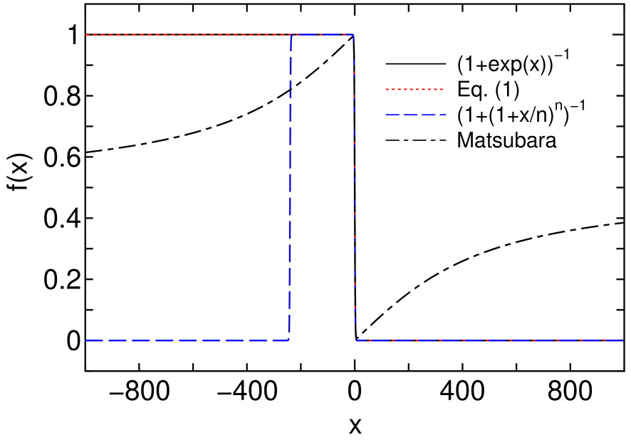
Figure 1: (Color online) The Fermi-Dirac function and its approximants as a function of the real axis . For substantial comparison all the approximants possess the same number of poles, 120 poles.
Now I consider the termination of the continued fraction Eq. (1) to a finite level , and assume is an even number, i.e., . It can be pointed out that Eq. (1) with the finite continued fraction may correspond to the Padé approximant of the Fermi-Dirac function itself rather than the exponential function, where and are relevant polynomials of M-th order. Thus, is zero up to -th order of , where is the Taylor series of the Fermi-Dirac function.[19] In this sense the proposed method is similar to the integral representation of the Fermi-Dirac function proposed by Goedecker,[11] while the overall feature of the derivation looks very different. In case of , for instance, Eq. (1) with the finite continued fraction is decomposed into partial fractions via the Padé approximant as follows:
| (2) |
In general, for the finite continued fraction terminated at , the Fermi-Dirac function can be approximated by the sum of partial fractions with the poles and residues as follows:
| (3) |
The expression becomes exact in case of the limit: . Noting that and is an odd function, it is found that the poles are symmetrically located on the complex plane with respect to the real axis. Furthermore, it will be shown in later discussion that the poles are located on only the imaginary axis and that the residues are real numbers. Thus, note that is a real number in Eq. (3). In case of an odd number of , an additional term which is proportional to is added to Eq. (3), and I will not discuss the odd case in this paper.
Although and may be analytically expressed for any termination to arbitrary order of , however, the formulae tend to be overly complicated to handle as increases. Thus, I present an alternative method of finding these values by introducing an eigenvalue problem. Taking account of a fact that the (1,1) element of the inverse of a tridiagonal matrix defined by
| (4) |
is given by
| (5) |
and comparing the continued fraction in the parenthesis of the right hand side of Eq. (1) with Eq. (5), the matrix elements of can be determined as follows:
| (6) | |||
| (7) |
where runs from 1 to for , and from 1 to for and . Thus, one obtains an interesting relation that the Fermi-Dirac function can be expressed by the (1,1) element of the resolvent of :
| (8) |
with
| (9) |
and
| (10) |
where and are matrices of in size, and Eq. (8) becomes exact as increases. The relation Eq. (8) tells us that finding the singular points of Eq. (1) is equivalent to solving the generalized eigenvalue problem , where is the eigenvector. Moreover, replacing with yields . Then, it can be proven that the eigenvalue is a pure imaginary number, giving that is a real number in Eq. (3), since is a real number due to the symmetric real matrices and .[20] The imaginary eigenvalues go away from the real axis and the distribution becomes sparse as the distance between the pole and the real axis increases as shown in the inset of Fig. 2, and this is a key feature for the fast convergence in the integrations of the Green function as shown later, since the Green function becomes structureless, while going away from the real axis. In addition, noting that the residue calculated from the eigenvectors for is a real number, since the eigenvectors consist of real numbers, and that
| (11) | |||||
one can find that the residue in Eq. (3) is a real number, where and appearing in the first line of Eq. (11) are due to the symmetry of . Thus, the poles and residues in Eq. (1) can be easily obtained by solving the eigenvalue problem with the real symmetric matrices and without any numerical difficulty.[21]
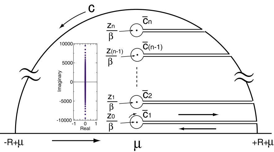
Figure 2: The path of the contour integration associated with Eq. (1). The inset shows the distribution of zero points of Eq. (1).
The characteristic feature of Eq. (1) that the poles are located on the imaginary axis and the residues are real is similar to that of the Matsubara summation. It is noted that the Fermi-Dirac function in the Matsubara summation is expressed by a development:
| (12) |
with the poles and the residues . This relation Eq. (12) can be derived by taking account of Eq. (A.10) and the Mittag-Leffler expansion [22] for . Therefore, one may think that their convergence properties should be comparable to each other. However, it will be shown later that the continued fraction representation by Eq. (1) provides a remarkable convergence speed compared to the Matsubara summation. The roots of the rapid convergence lies on an interesting non-uniform distribution of the poles on the imaginary axis. It is observed from Fig. 3 that in case of the interval between neighboring poles of Eq. (1) are uniformly located up to around 61th poles with the same interval as that of the Matsubara poles, and from then onward it increases very rapidly as the distance between the pole and the real axis increases, while the Matsubara poles distribute uniformly on the imaginary axis everywhere. The distribution of the poles seems to be almost independent of the number of poles , provided that the pole index is normalized by the number of poles on the upper half complex plane, i.e., the interval starts to increase rapidly at about 61 % of the total number of poles . The sparse distribution of poles of Eq. (1) in the faraway region from the real axis well matches the fact that the Green function becomes a smooth function, while going away from the real axis, and by covering a wide range of the imaginary axis with a small number of poles, the continued fraction representation Eq. (1) can reproduce very well the Fermi-Dirac function on the real axis as shown in Fig. 1. The property is the reason why Eq. (1) is much superior to the Matsubara summation for the integration of the Green function.
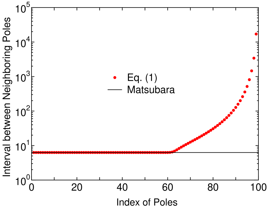
Figure 3: (Color online) The interval between neighboring poles of Eq. (1) terminated at as a function of an index of poles, where the index of poles is determined in ascending order with respect to the absolute value of poles. The interval for the Matsubara poles is .
2.2 Calculation of the density matrix
We are now ready to make full use of Eq. (3) to evaluate integrated quantities associated with a Green function with the Fermi-Dirac function. Here, as an example, I consider evaluation of the one-particle density matrix , which is one of the most important quantities in electronic structure calculations, calculated by the Green function being an analytic function apart from the real axis with the Fermi-Dirac function. Considering the expression of Eq. (3) and the contour integral with an integration path on the upper half complex plane as shown in Fig. 2, the density matrix can be evaluated by
| (13) | |||||
where the factor 2 in the first line is for spin multiplicity, , the zeroth order moment of the Green function, and a positive infinitesimal. This expression Eq. (13) is valid for Green functions such as and , where and are real symmetric Hamiltonian and overlap matrices, and is an energy-dependent matrix such as a self-energy matrix which is real symmetric on the real axis. A more general case with energy dependent complex matrices is discussed in the Appendix B. The first term in the second line of Eq. (13) is transformed into the zeroth order moment of the Green function by the contour integration as follows:
| (14) |
Although the evaluation of the second term in the final line of Eq. (13) is straightforward, the calculation of the first term is nontrivial. However, it is shown that the zeroth order moment can be easily evaluated by utilizing the moment representation of the Green function as shown below. Starting from the Lehmann representation of the Green function and taking account of for , one can obtain the moment representation of the Green function:
| (15) |
where is the th moment of the Green function defined by
| (16) |
On the other hand, multiplying the both side of Eq. (15) by and integrating from to along the real axis with an infinitesimal imaginary part , one has an alternative expression for the moment:
| (17) |
It is found that the case of in Eq. (17) corresponds to Eq. (14). Writing in Eq. (15), assuming that is large enough so that the terms associated with higher orders of can be negligible, and taking , one can obtain an approximate expression for :
| (18) |
where is a large real number and 1.0e+10 is used in this study. Therefore, one can see that just one evaluation of the Green function yields the zeroth order moment . In Eq. (13) the integration on the real axis is transformed into a quadrature on an axis perpendicular to the real axis with the characteristic distribution of the poles except for the evaluation of the zeroth moment . Thus, it is reasonable to anticipate that the density matrix evaluated by Eq. (13) quickly converges as a function of the number of poles, since the Green function becomes structureless by going away from own poles located on the real axis.
2.3 In case of a general density matrix
In this subsection an expression is given for the evaluation of a general density matrix defined by
| (19) |
where it is assumed that the Green function possesses the same property as discussed for Eq. (13). It is worth mentioning that is a conventional density matrix given by Eq. (13), and is the so called energy density matrix. Noting that , and taking account of Eq. (3), one has the following expression:
| (20) |
This expression becomes exact in case of . Therefore, putting Eq. (20) into Eq. (19) and considering a contour integration with the same path given by Fig. 2 as discussed for Eq. (13), we see that can be evaluated by
| (21) |
with
| (22) |
The moments up to th orders in Eq. (21) can be evaluated by generalizing the way of calculating discussed in the previous subsection. If the summation in the moment representation Eq. (15) of the Green function is terminated at the th level, the moments up to th orders can be determined by solving a linear equation for each element (i,j):
| (23) |
where are large complex numbers, and can be given by with a large , while they can be chosen arbitrarily only if is large enough so that the higher order terms can be negligible. Thus, one can see that the general density matrix is evaluated by the proposed method as well as the conventional density matrix. In the Appendix C the integrations of the Green function with the derivative of the Fermi-Dirac function with respect to energy are discussed.
3 NUMERICAL RESULTS
To demonstrate the rapid convergence of the proposed method I give two numerical examples, (i) calculation of the density matrix for a simple model Green function and (ii) a total energy calculation of aluminum bulk in the face centered cubic (FCC) structure within the Harris density functional.[23]
As a simple model, let us consider a model Green function given by
| (24) |
where the unit of energy is in eV. It is assumed that the chemical potential is 0 eV and that the electronic temperature is 300 K. Table 1 show the density matrix calculated by three method: the proposed method through Eq. (13), the method discussed in Ref. [10], and the Matsubara summation.[15] We see that the density matrix calculated by the proposed method rapidly converges at the analytic value (3.0) using only 40 poles, while the convergence speed by the second method is about three times slower than that of the proposed method. Also, the stepwise improvement of the density matrix in the second method is attributed to the plunge step of the approximate function used in the method in the lower energy region as shown in Fig. 1. It is also confirmed that the convergence of the Matsubara summation is quite slow.
| Poles | Proposed | Matsubara | |
|---|---|---|---|
| 10 | 2.897457365704 | 0.000000000704 | 2.268430836092 |
| 20 | 2.999785910601 | 0.938582044963 | 2.424349652146 |
| 30 | 2.999999992975 | 1.000000000000 | 2.520372160464 |
| 40 | 3.000000000000 | 1.000000000001 | 2.588358024187 |
| 60 | - | 2.000000000000 | 2.681479492145 |
| 80 | - | 2.000000000000 | 2.742612466824 |
| 100 | - | 2.999998800183 | 2.785347036205 |
| 120 | - | 3.000000000000 | 2.816567540132 |
| 200 | - | - | 2.885375367071 |
| 500 | - | - | 2.953166094829 |
| 5000 | - | - | 2.995297020881 |
As well as the simple model, I show in Table 2 the convergence of the total energy calculated by the recursion method [5] with the Harris functional[23] for FCC aluminum as a function of the number of poles. In this calculation I use pseudo-atomic double valence numerical functions as basis set,[24] a norm-conserving pseudopotential,[25] and a generalized gradient approximation (GGA) to the exchange-correlation potential.[26] The Green function is evaluated by the recursion method with ten recursion levels.[5] Also, an electronic temperature of 600 K is used. The DFT calculation was done using the OpenMX code.[27] As shown in Table 2, it is obvious that the proposed method provides remarkable rapid convergence. The use of only 80 poles yields the convergent result of 14 digits which corresponds to the limit of double precision. On the other hand, it turns out that the second and third methods are much slower than the proposed method, and that the full convergence is not achieved even in case of ten thousands poles. It is also worth mentioning that the proposed method can be applicable to insulators and semi-conductors as well as metallic systems without depending the magnitude of band gap in a system if the Fermi energy is determined so that the total number of electrons in the whole system can be conserved.
| Poles | Proposed | Matsubara | |
|---|---|---|---|
| 10 | -42.933903047211 | -33.734015919550 | -39.612354360046 |
| 20 | -47.224346653790 | -33.623477214678 | -39.849746603905 |
| 40 | -48.323790725570 | -33.346245616679 | -40.216055898502 |
| 60 | -48.324441992259 | -33.143128624551 | -39.676965494522 |
| 80 | -48.324441994952 | -32.870752577236 | -43.523770052176 |
| 150 | -48.324441994952 | -33.837428496424 | -41.836938942518 |
| 200 | - | -33.418012271726 | -42.543354202255 |
| 250 | - | -34.003411636691 | -43.024756221080 |
| 300 | - | -34.003236479262 | -43.466729654170 |
| 350 | - | -48.324440028792 | -43.834528739677 |
| 400 | - | -48.324440274509 | -44.185100655185 |
| 600 | - | -48.324440847749 | -45.233651519749 |
| 1000 | - | -48.324441306517 | -46.331692884149 |
| 2000 | - | -48.324441650693 | -47.202779497545 |
| 5000 | - | -48.324441857239 | -47.921384128418 |
| 10000 | - | -48.324441926094 | -48.122496320516 |
4 CONCLUSIONS
I have developed an efficient contour integration method for electronic structure calculation methods based on the Green function. By introducing a continued fraction representation of the Fermi-Dirac function, the integration of Green function with the Fermi-Dirac function on the real axis is transformed into a quadrature on an axis perpendicular to the real axis except for the evaluation of the moments. Although the feature is similar to that of the Matsubara summation, the most important distinction between those lies on the distribution of poles. The poles of the continued fraction distribute uniformly on an axis perpendicular to the real axis with the same interval as the Matsubara poles up to about 61 % of the total number of poles, and from then onward the interval between neighboring poles increases rapidly as the poles go away from the real axis, while the Matsubara poles are uniformly located on an axis perpendicular to the real axis. The characteristic distribution of poles in the continued fraction well matches the smoothness of the Green function in the distant region from the real axis, and therefore enables us to achieve the remarkable convergence using a small number of poles. The numerical examples clearly demonstrate the computational efficiency and accuracy of the proposed method. Since the contour integration by the continued fraction representation can be regarded as a natural generalization of the Matsubara summation with respect to the distribution of poles, it is anticipated that the proposed method can be applied to not only the electronic structure calculation methods, but also many other applications.
Acknowledgments
The author was partly supported by CREST-JST and the Next Generation Super Computing Project, Nanoscience Program, MEXT, Japan.
Appendix A Derivation of the continued fraction representation of the Fermi-Dirac function
In this Appendix the continued fraction representation Eq. (1) of the Fermi-Dirac function is derived using a hypergeometric function. The generalized hypergeometric function is defined as a power series expansion by
| (A.1) |
with
| (A.2) |
where is the Pochhammer symbol defined by
| (A.3) |
with an exceptional definition of in case of . The special cases of Eq. (A.1) yield the following relations:
| (A.4) |
| (A.5) |
For later discussion, I will drop the suffixes of the hypergeometric function for simplicity of notation, and define to be . Furthermore, let us introduce a recurrence relation for :
| (A.6) |
This relation can be proven by comparing the term in the power series piece by piece. Dividing both the sides of Eq. (A.6) by and considering the reciprocal, one has
| (A.7) |
Replacing the ratio of in the right hand side of Eq. (A.7) by Eq. (A.7) with increment of by one recursively, one can obtain the following continued fraction:
| (A.8) |
Now can be expressed by a continued fraction using Eqs. (A.4), (A.5), and (A.8) as follows:
| (A.9) | |||||
Noting that , one has
| (A.10) | |||||
Inserting Eq. (A.9) into Eq. (A.10) yields the continued fraction representation Eq. (1) of the Fermi-Dirac function.
Appendix B In case of the Green function consisting of complex matrices
If the Green function consists of energy dependent complex matrices, a more general expression, different from Eq. (13), is used to calculate the density matrix. As such a case, here let us assume that the Green function consists of matrices depending on energy and k-point , i.e.,
| (B.1) | |||||
where and are complex and real variables, respectively, and the second and third lines are the Lehmann and moment representations of the Green function. It is assumed that poles of the Green function Eq. (B.1) are located on the real axis, which is verified at least in case the self-energy matrix is calculated using the surface Green function.[6] Considering that off-diagonal elements of are complex in general, the density of states depending on is given using both the retarded and advanced Green functions, and , by
| (B.2) |
where the factor 2 due to spin multiplicity was considered. Thus, the density matrix can be evaluated by
| (B.3) | |||||
where is the volume of the unit cell, represents the integration over the first Brillouin zone, and and are defined by
| (B.4) | |||||
| (B.5) |
Thus, we see that from the Green function defined by Eq. (B.1) the density matrix can be easily evaluated using the proposed method, since and are computed in the same way as for Eq. (13) by considering the contour integrals in the upper and lower complex planes, respectively.
Appendix C In case of the derivative of the Fermi-Dirac function
The calculations of physical quantities such as electric and thermal conductances require integrals with the derivative of the Fermi-Dirac function with respect to energy. In the Appendix I give the outline for applying the proposed method to such cases. By making use of the continued fraction representation Eq. (1) of the Fermi-Dirac function, the derivative of the Fermi-Dirac function can be expressed as follows:
| (C.1) | |||||
where , , and is given by
| (C.2) |
It is found from Eq. (C.1) that the derivative of the Fermi-Dirac function approximated by the finite continued fraction possesses the second order poles of the continued fraction as well as the first order poles. Therefore, if the Green function is analytic around the pole, by Taylor expanding it at the pole as
| (C.3) |
one has to include contributions of the derivative of the Green function with respect to energy which can be evaluated through a response function calculated from the Green functions.
References
- [1] J. Korringa, Physica 13, 392 (1947).
- [2] W. Kohn and N. Rostoker, Phys. Rev. 94, 1111 (1954).
- [3] N. Papanikolaou, R. Zeller, and P. H. Dederichs, J. Phys.: Condens. Matter 14, 2799 (2002).
- [4] R. Haydock, V. Heine, and M.J. Kelly, J. Phys. C 5, 2845 (1972); 8, 2591 (1975); R. Haydock, Solid State Phys. 35, 216 (1980).
- [5] T. Ozaki and K. Terakura, Phys. Rev. B 64, 195126 (2001).
- [6] M.P. Lopez Sancho, J.M. Lopez Sancho, J.M.L. Sancho, and J. Rubio, J. Phys. F 15, 851 (1985).
- [7] J. Inglesfield, J. Phys. C 14, 3795 (1981).
- [8] L. Hedin, Phys. Rev. A 139, 796 (1965).
- [9] F. Aryasetiawan and O. Gunnarsson, Rep. Prog. Phys. 61, 237 (1998).
- [10] D.M.C. Nicholson, G.M. Stocks, Y. Wang, W.A. Shelton, Z. Szotek, and W.M. Temmerman, Phys. Rev. B 50, 14686 (1994).
- [11] S. Goedecker, Phys. Rev. B 48, 17573 (1993).
- [12] K. Wildberger, P. Lang, R. Zeller, and P.H. Dederichs, Phys. Rev. B 52, 11502 (1995).
- [13] V. Drchal, J. Kudrnovský, P. Bruno, I. Turek, P.H. Dederichs, and P. Weinberger, Phys. Rev. B 60, 9588 (1999).
- [14] F. Gagel, J. Comput. Phys. 139, 399 (1998).
- [15] T. Matsubara, Prog. Theor. Phys. 14, 351 (1955).
- [16] G. D. Mahan, Many Particle Physics, (Plenum, New York, 1981).
- [17] In addition to Eq. (1), I investigated the convergence properties of other continued fraction representations of the Fermi-Dirac function, which are given in Ref. [18], and it turned out that Eq. (1) is the best convergent approximant among these continued fraction representations. However, there is a possibility of further improvement for the convergence of the continued fraction representation, e.g., a continued fraction derived from a multipoints Padé approximant.
- [18] L. Lorentzen and H. Waadeland, Continued Fractions with Applications, Amsterdam, Netherlands: North-Holland, 1992.
- [19] Although the rigorous proof remains unavailable, I confirmed validity of the statement for the cases up to by MATHEMATICA.
- [20] Consider an eigenvalue problem having the same eigenvalues and eigenvectors as for , where and . Noting that is positive definite, the eigenvalue problem can be transformed into , where is a diagonal matrix of which diagonal elements are the inverse of square root of the corresponding diagonal element of , and . If the dimension of is an even number , the determinant of is , while it is zero in case of an odd number, in this case is a well defined real symmetric matrix. Thus, it is found that the eigenvalues and eigenvectors of are purely real, provided that the dimension of is an even number .
- [21] Tables for the poles and residues, and a program code of generating those are freely available on a web site (https://www.openmx-square.org/zero_fermi/zero_fermi.html) under the term of GNU-GPL.
- [22] I.S. Gradshtein, I.M. Ryzhik, Table of integrals, series, and products, A. Jeffrey, Ed. (Academic Press, New York, 1980).
- [23] J. Harris, Phys. Rev. B 31, 1770 (1985).
- [24] T. Ozaki, Phys. Rev. B. 67, 155108 (2003); T. Ozaki and H. Kino, ibid. 69, 195113 (2004).
- [25] N. Troullier and J.L. Martins, Phys. Rev. B 43, 1993 (1991).
- [26] J.P. Perdew, K. Burke, and M. Ernzerhof, Phys. Rev. Lett. 77, 3865 (1996).
- [27] The code, OpenMX, pseudo-atomic basis functions, and pseudopotentials are available on a web site (http://www.openmx-square.org/).