Fast spherical Bessel transform via fast Fourier transform and recurrence formula
Masayuki Toyoda and Taisuke Ozaki
Research Center for Integrated Science,
Japan Advanced Institute of Science and Technology,
1-1, Asahidai, Nomi, Ishikawa 932-1292, Japan
Copyright 2009 Elsevier B.V.
This article is provided by the author for the reader's personal use only.
Any other use requires prior permission of the author and Elsevier B.V.
NOTICE: This is the authorÅfs version of a work accepted for publication by Elsevier.
Changes resulting from the publishing process, including peer review, editing,
corrections, structural formatting and other quality control mechanisms, may
not be reflected in this document. Changes may have been made to this work
since it was submitted for publication. A definitive version was subsequently
published in Computer Physics Communications 181, 277-282 (2010),
DOI: 10.1016/j.cpc.2009.09.020 and may be found at
http://dx.doi.org/10.1016/j.cpc.2009.09.020.
Abstract
We propose a new method for the numerical evaluation of the
spherical Bessel transform.
A formula is derived for the transform by using an integral
representation of the spherical Bessel function and by changing
the integration variable.
The resultant algorithm consists of a set of the Fourier
transforms and numerical integrations over a linearly spaced
grid of variable  in Fourier space.
Because the
in Fourier space.
Because the  -dependence appears in the upper limit of the
integration range, the integrations can be performed effectively
in a recurrence formula.
Several types of atomic orbital functions are transformed with
the proposed method to illustrate its accuracy and efficiency,
demonstrating its applicability for transforms of general order
with high accuracy.
-dependence appears in the upper limit of the
integration range, the integrations can be performed effectively
in a recurrence formula.
Several types of atomic orbital functions are transformed with
the proposed method to illustrate its accuracy and efficiency,
demonstrating its applicability for transforms of general order
with high accuracy.
Keywords: Hankel transforms, spherical Bessel functions, atomic orbitals
PACS: 02.30.Uu, 71.15.Ap, 31.15.-p
Introduction
Numerical evaluation of integrals containing the spherical Bessel
function is of importance in many fields of computational science
and engineering
since the spherical Bessel function is often used as the
eigenfunction for spherical coordinate systems.
The integrals are known as the spherical Bessel transform
(SBT) which is classified into a more general family of the
Hankel or Fourier-Bessel transforms.
The SBT is involved in many physical problems such as
the scattering in atomic or nuclear systems [1,2],
the simulation of the cosmic microwave background [3],
and the interaction of electrons in molecules and crystals
[4,5].
Several computational methods have been developed for the Hankel
transforms [6,7,8].
However, not many of them can be applied for SBT.
There have been proposed three different approaches for SBT for
general order:
(a) recasting the transform integral as a convolution integral
by changing the coordinate variables [9,10,11],
(b) expansion in terms of a series of Fourier cosine and
sine transforms by the trigonometric expansion of the spherical
Bessel function [12],
and (c) the discrete Bessel transform method which describes
SBT as an orthogonal transform [13].
The approach (a) is quite fast since it utilizes the fast Fourier
transform (FFT) algorithm.
The computation time actually scales as
 , where
 is the number of quadrature points.
It, however, has a major drawback caused by the logarithmic
grid that almost all the grid points are located in
close proximity of the origin.
The computation time of the approach (b) which also uses FFT
scales as
is the number of quadrature points.
It, however, has a major drawback caused by the logarithmic
grid that almost all the grid points are located in
close proximity of the origin.
The computation time of the approach (b) which also uses FFT
scales as
 , where
  is the order
of transform.
Therefore, it becomes slower for the higher order transform.
In addition to that, since it requires the integrand to be
multiplied by inverse powers of the radial coordinate,
the high order transforms may become unstable.
The computation time of the approach (c) scales as
is the order
of transform.
Therefore, it becomes slower for the higher order transform.
In addition to that, since it requires the integrand to be
multiplied by inverse powers of the radial coordinate,
the high order transforms may become unstable.
The computation time of the approach (c) scales as  .
The quadrature points are located at each zero of the spherical
Bessel function.
The optimized selection of the quadrature points enables us to
use a small number of
.
The quadrature points are located at each zero of the spherical
Bessel function.
The optimized selection of the quadrature points enables us to
use a small number of  while keeping the accuracy of the
computation.
However, when consecutive transforms with different orders
are required, it may become a minor trouble that the optimized
quadrature points differ depending on the order of transform.
while keeping the accuracy of the
computation.
However, when consecutive transforms with different orders
are required, it may become a minor trouble that the optimized
quadrature points differ depending on the order of transform.
In this paper, we propose a new method for the numerical SBT
which uses a linear coordinate grid.
The transform is decomposed into the Fourier transforms and
the numerical integrations which can be evaluated recursively.
The computation time for the present method scales as
 with overhead for the numerical integration
which scales as
with overhead for the numerical integration
which scales as  .
The linear coordinate grid prevents us from troubles
caused by the non-uniform or order-dependent grid points.
If the considered problem requires to transform a function with
various orders, the present method has further the advantage that
the results of the most time consuming calculations
(i.e. the Fourier transforms and the integrations)
for a transform with a certain order
.
The linear coordinate grid prevents us from troubles
caused by the non-uniform or order-dependent grid points.
If the considered problem requires to transform a function with
various orders, the present method has further the advantage that
the results of the most time consuming calculations
(i.e. the Fourier transforms and the integrations)
for a transform with a certain order  can also be used for
transforms with any order less than
can also be used for
transforms with any order less than  .
.
Formulation
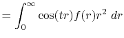
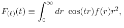
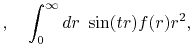
We are interested in the  -th order SBT of a function
 which is defined as follows:
 |
(1) |
where  is the spherical Bessel function of the
first kind.
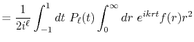
The integral representation of the spherical Bessel function
is given by
is the spherical Bessel function of the
first kind.
The integral representation of the spherical Bessel function
is given by
 |
(2) |
where  is the Legendre polynomials
Here,  is the double factorial
 |
(5) |
with an exceptional definition that
 .
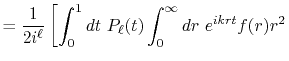
By substituting Eq. (2) into Eq. (1),
and using the parity property
.
By substituting Eq. (2) into Eq. (1),
and using the parity property
 ,
the transform is rewritten as follows:
,
the transform is rewritten as follows:
Now, we change the variables as  , and it becomes
 |
(7) |
where
 is the Fourier cosine/sine transform
of
is the Fourier cosine/sine transform
of  ,
,
and
 is the largest integer that does not
exceed
is the largest integer that does not
exceed  .
Finally, by expanding the Legendre polynomials, the transform
is decomposed into a sum of definite integrals
.
Finally, by expanding the Legendre polynomials, the transform
is decomposed into a sum of definite integrals 
where  is given by
 |
(11) |
Since the integrals  appearing in Eqs.
(9) and (10) have
the same parity as the order of transform
appearing in Eqs.
(9) and (10) have
the same parity as the order of transform  , either the
Fourier cosine or sine transform is required to be performed,
for given
, either the
Fourier cosine or sine transform is required to be performed,
for given  .
In our implementation, as explained later, at most two more
Fourier transforms are required to be performed to
evaluate the derivatives of
.
In our implementation, as explained later, at most two more
Fourier transforms are required to be performed to
evaluate the derivatives of
 .
Therefore, regardless of the order of transform, only three
Fourier transforms are required.
On the other hand, since the integrals
.
Therefore, regardless of the order of transform, only three
Fourier transforms are required.
On the other hand, since the integrals  depend on the
order of transform through
depend on the
order of transform through  terms,
a number of
terms,
a number of  different integrals are required for
the summation in Eqs. (9) and
(10).
Even so, however, this does not increase the computational
cost because
different integrals are required for
the summation in Eqs. (9) and
(10).
Even so, however, this does not increase the computational
cost because  does not appear in the integrand of Eq.
(11) and thus the computation cost
for
does not appear in the integrand of Eq.
(11) and thus the computation cost
for  scales as
  , rather
than as
, rather
than as  .
.
Implementation
In order to avoid problems arising from  at the origin,
we define the
at the origin,
we define the  - and
- and  -grid points at half-interval shifted
positions as follows:
-grid points at half-interval shifted
positions as follows:
At each point of  , the integral
  is divided into
its segments
is divided into
its segments
 |
(14) |
where the segments are defined as
By defining the sum of the segments as
 ,
the following simple recurrence formula is obtained:
,
the following simple recurrence formula is obtained:
Therefore, the evaluation of the integral is accomplished for
all the  -grid points through a summation of segments
  ,
where, at each step of the summation, the subtotal
,
where, at each step of the summation, the subtotal  divided by
  gives
gives  .
.
Each segment is evaluated by locally interpolating
 with a polynomial curve.
Since no grid point is available in between the both ends of
the integration range, the derivatives of
with a polynomial curve.
Since no grid point is available in between the both ends of
the integration range, the derivatives of
 are also
required to interpolate with higher order polynomials.
By noting that only the trigonometric functions depend on
are also
required to interpolate with higher order polynomials.
By noting that only the trigonometric functions depend on  in the integrand of (8),
the derivatives and second derivatives are obtained analytically
as follows:
in the integrand of (8),
the derivatives and second derivatives are obtained analytically
as follows:
By interpolating
 with a
  -th order polynomial,
the integral segments are given by
-th order polynomial,
the integral segments are given by
where the coefficients  are determined from the values
and derivatives of
are determined from the values
and derivatives of
 at
at  and
and
 (see Appendix A).
We have performed the interpolation with linear (
(see Appendix A).
We have performed the interpolation with linear ( ), cubic (
 ),
and quintic (
),
and quintic ( ) polynomials.
Since a higher order interpolation suffers more severely from
the arithmetic errors, interpolations with a polynomial of
order
) polynomials.
Since a higher order interpolation suffers more severely from
the arithmetic errors, interpolations with a polynomial of
order  have not been tested.
To summarize, the present method computes the transform of
a function  with the order
  via the following steps:
- Fourier cosine/sine transforms of
 multiplied by a power
of
multiplied by a power
of  (Eqs. (8), (19), and (20)).
- Evaluation of the integral segments
 by the piecewise polynomial interpolation.
(Eq. (21)).
by the piecewise polynomial interpolation.
(Eq. (21)).
- Evaluation of
 through the summation of
  (Eqs. (17) and (18)).
- Weighted summation of
 to give the transformed function
 (Eqs. (9) and (10)).
The order of transform explicitly appears only in the final
step.
Therefore, once a transform with an order  is performed,
then one can also perform another transform with another order
is performed,
then one can also perform another transform with another order
 by repeating only the final step and skipping
the others.
The computation cost for the first step is
by repeating only the final step and skipping
the others.
The computation cost for the first step is
 ,
where
,
where  is the required number of the Fourier transforms.
If the quintic interpolation is used and a transform with one
specific order is required,
is the required number of the Fourier transforms.
If the quintic interpolation is used and a transform with one
specific order is required,  , as mentioned before, while
 if transforms with various orders are required.
The computation cost for the second and third steps scales
as
if transforms with various orders are required.
The computation cost for the second and third steps scales
as  because of the use of the recurrence formula.
It is, however, multiplied by the overhead due to the polynomial
interpolation which depends on the order of interpolation
because of the use of the recurrence formula.
It is, however, multiplied by the overhead due to the polynomial
interpolation which depends on the order of interpolation  .
The computation cost for the final step is
.
The computation cost for the final step is
 .
.
Computation results
The present method has been applied in transforming the
atomic orbital wave functions which are used in quantum
chemistry and condensed matter physics.
Three types of atomic orbitals have been examined:
the Gaussian-type orbital (GTO), the Slater-type orbital
(STO), and the numerically defined pseudo-atomic orbital
(PAO) functions.
The first two functions are good examples to investigate
in detail the numerical error accompanied by the present
method since the exact form of the transformed function
is available,
while the PAO function, being strictly localized within
a certain radius, is another example to check
the applicability of the method for non-analytic functions.
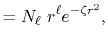
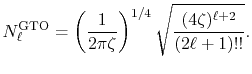
The normalized GTO function in spherical coordinate is
defined as follows:
 |
 |
(22) |
where the normalization factor is given by
 |
(23) |
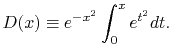
The corresponding transformed function is
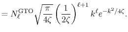
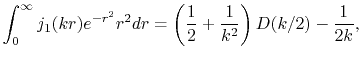
Figure 1 (a) shows the the numerical error in
the present method in the 0th-order transform of the GTO function,
where the integral segments  have been evaluated by interpolating
 with the linear
(solid line), cubic (dashed line), and quintic
(dash-dotted line) polynomials.
The parameters used in the calculation are as follows:
the exponent of GTO
with the linear
(solid line), cubic (dashed line), and quintic
(dash-dotted line) polynomials.
The parameters used in the calculation are as follows:
the exponent of GTO  , the number of grid points
 , and the maximum value of
  -grid
-grid
 .
It is clearly observed that the error is reduced quickly
as the order of interpolation polynomial increases, and
that the quintic polynomial gives a sufficiently accurate
result.
In Fig. 1 (b), the numerical error for the
15th-order transform of GTO is shown, where the same
parameters as the previous calculation and the quintic
polynomial interpolation is used.
Even in such a high order transform, the error remains small.
This implies that the numerical error comes mainly from the
integration of the segments while the possible rounding-off
error in Eqs. (9), (10),
and (11) is actually negligible
unlike in the approach (b) referred in the introduction
of this paper [12].
.
It is clearly observed that the error is reduced quickly
as the order of interpolation polynomial increases, and
that the quintic polynomial gives a sufficiently accurate
result.
In Fig. 1 (b), the numerical error for the
15th-order transform of GTO is shown, where the same
parameters as the previous calculation and the quintic
polynomial interpolation is used.
Even in such a high order transform, the error remains small.
This implies that the numerical error comes mainly from the
integration of the segments while the possible rounding-off
error in Eqs. (9), (10),
and (11) is actually negligible
unlike in the approach (b) referred in the introduction
of this paper [12].
Figure 1:
(a) Numerical error accompanied by the 0th-order transform of the GTO function ( ), where the linear (solid line), cubic (dashed line), and quintic (dash-dotted line) polynomial interpolations are used to evaluate integrals.
(b) Numerical error accompanied by the 15th-order transform of the GTO function
(
), where the linear (solid line), cubic (dashed line), and quintic (dash-dotted line) polynomial interpolations are used to evaluate integrals.
(b) Numerical error accompanied by the 15th-order transform of the GTO function
( ), where the quintic polynomial interpolation is used to
evaluate integrals.
), where the quintic polynomial interpolation is used to
evaluate integrals.
|
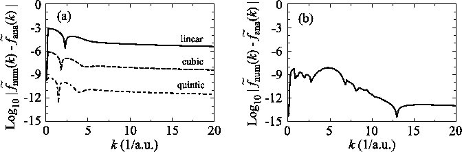
Since the numerical error in the integration of a segment
remains in the summation in Eq. (14),
the numerical error of the segments in the small- region
also contributes to the error in the large-
region
also contributes to the error in the large- region.
This explains why the damping of the error at large-
region.
This explains why the damping of the error at large- region is
so slow in Fig. 1 (a).
A downward summation is effective to reduce this error.
In Fig. 2, the numerical error in
the 0th-order transform of GTO is plotted, where the summation
of the segments are performed upward (solid line) and downward
(dashed line).
In the downward summation, the numerical error in the large-
region is
so slow in Fig. 1 (a).
A downward summation is effective to reduce this error.
In Fig. 2, the numerical error in
the 0th-order transform of GTO is plotted, where the summation
of the segments are performed upward (solid line) and downward
(dashed line).
In the downward summation, the numerical error in the large- region becomes much smaller, while, in the small-
 region,
the error becomes larger because of the accumulation of the
error from the large-
region,
the error becomes larger because of the accumulation of the
error from the large- region.
Therefore, by connecting the results of the upward and downward
summations at a certain
region.
Therefore, by connecting the results of the upward and downward
summations at a certain  point (for example,
  = 5),
accurate results can be obtained in both small- and large-
= 5),
accurate results can be obtained in both small- and large- regions.
Figure 2:
Numerical error accompanied by the 0th-order transform of the GTO function
( ), where the upward (solid line) and downward (dashed line)
summations are used.
), where the upward (solid line) and downward (dashed line)
summations are used.
|
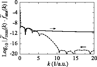
Figure 3:
Numerical error accompanied by the 1st-order transform of the GTO function
( ), where the quintic polynomial interpolation and the upward
summation are used.
The calculations are performed with various
), where the quintic polynomial interpolation and the upward
summation are used.
The calculations are performed with various  , namely, 128 (solid line),
256 (dashed line), 512 (dash-dotted line), and 1024 (dotted line),
while keeping
, namely, 128 (solid line),
256 (dashed line), 512 (dash-dotted line), and 1024 (dotted line),
while keeping
 .
.
|
So far, the transforms have been performed where the order of
transform  and the order of the GTO function
  are
equivalent.
In Fig. 3, the numerical error
in the transform with the order
are
equivalent.
In Fig. 3, the numerical error
in the transform with the order  for the GTO function
whose order is
for the GTO function
whose order is  is plotted with a variety of grid
spacings in real space.
It is found that the error (solid line) is larger than that of
the case
is plotted with a variety of grid
spacings in real space.
It is found that the error (solid line) is larger than that of
the case
 calculated with the same condition
(dash-dotted line in Fig. 1 (a)).
The decrease of the error by smaller grid spacing implies that
fine grid spacing is necessary for the accurate sine transform
in Eq. (8) since the GTO function of the order
calculated with the same condition
(dash-dotted line in Fig. 1 (a)).
The decrease of the error by smaller grid spacing implies that
fine grid spacing is necessary for the accurate sine transform
in Eq. (8) since the GTO function of the order  has
a finite value at
has
a finite value at  while the spherical Bessel function
of the order
while the spherical Bessel function
of the order  vanishes proportionally to
  .
The different behaviors near the origin results in another
undesirable fact that the transformed function in Fourier space
has a very long tail.
In the case considered here, the analytic form of the SBT of the
GTO function is given as
.
The different behaviors near the origin results in another
undesirable fact that the transformed function in Fourier space
has a very long tail.
In the case considered here, the analytic form of the SBT of the
GTO function is given as
 |
(25) |
where  is the Dawson's integral [14] which is defined as
 |
(26) |
From the asymptotic form of the Dawson's integral, the SBT of the GTO function
is known to behave as
 |
(27) |
when  is large.
Therefore, in general, a wide range of
is large.
Therefore, in general, a wide range of  -grid has to be employed
where the orders of transform and the function are not equivalent.
-grid has to be employed
where the orders of transform and the function are not equivalent.
In quantum chemistry, the STO wave functions are often used
as the basis functions for the molecular orbitals.
The radial part of the STO functions is given by
 |
 |
(28) |
where the normalization factor is
 |
(29) |
The corresponding transformed function is given as
 |
(30) |
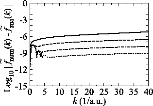
In Fig. 4,
plotted is the numerical error for the 0th- and 15th-order transforms
of STO.
The parameters used in the calculations are as follows:
the number of grid points  and the maximum value of the
 -grid
-grid
 (solid line in Fig. 4 (a));
  and
and
 (dashed line in Fig. 4 (a));
 and
and
 (solid line in Fig.
4 (b));
(solid line in Fig.
4 (b));  and
and
 (dashed line in Fig. 4 (b)).
The exponent of STO is
(dashed line in Fig. 4 (b)).
The exponent of STO is  for all the calculations.
There are two kinds of sources for the numerical error in the
SBT for STO: the cusp at the origin and the long tail of STO,
and they are illustrated in Fig. 4.
The use of the fine grid by increasing
for all the calculations.
There are two kinds of sources for the numerical error in the
SBT for STO: the cusp at the origin and the long tail of STO,
and they are illustrated in Fig. 4.
The use of the fine grid by increasing  reduces the error
as shown in Fig. 4 (a), which implies the
requirement of a fine grid near the cusp for the accurate
integration in Eq. (8).
On the other hand, the error is reduced by using the wide
range of
reduces the error
as shown in Fig. 4 (a), which implies the
requirement of a fine grid near the cusp for the accurate
integration in Eq. (8).
On the other hand, the error is reduced by using the wide
range of  -grid as shown in Fig. 4 (b)
because of the long tail of STO (
-grid as shown in Fig. 4 (b)
because of the long tail of STO ( ).
).
Figure 4:
(a) Numerical error accompanied by the 0th-order transform of the STO function
( ), where the following two configurations are used:
 ,
,
 , and
, and
 (solid line);
 ,
,
 , and
, and
 (dashed line).
The quintic interpolation and the upward summation are used.
(b)
Numerical error accompanied by the 15th-order transform of the STO function
(
(dashed line).
The quintic interpolation and the upward summation are used.
(b)
Numerical error accompanied by the 15th-order transform of the STO function
( ), where the following two configurations are used:
 ,
,
 , and
, and
 (solid line);
 ,
,
 , and
, and
 (dashed line).
The quintic interpolation and the upward summation are used.
(dashed line).
The quintic interpolation and the upward summation are used.
|
In the electronic structure calculations based on the density
functional theory (DFT), the non-analytic atomic orbitals are
often used as well as the analytic functions such as the GTO
and STO functions.
The PAO function is one of those non-analytic basis functions
and used in many  DFT calculation methods.
A PAO function is calculated by solving the atomic
Kohn-Sham equation with confinement pseudopotentials
[15].
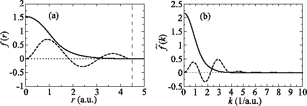
Figure 5 (a) shows the PAO functions of the
DFT calculation methods.
A PAO function is calculated by solving the atomic
Kohn-Sham equation with confinement pseudopotentials
[15].
Figure 5 (a) shows the PAO functions of the  and
and
 states of an oxygen atom, where the confinement
radius is
states of an oxygen atom, where the confinement
radius is  a.u.
The corresponding transformed functions are plotted
in Fig. 5 (b).
Since the mathematical formula for the forward and backward SBT is
equivalent except for an additional factor of
a.u.
The corresponding transformed functions are plotted
in Fig. 5 (b).
Since the mathematical formula for the forward and backward SBT is
equivalent except for an additional factor of  , the
function should recover the original shape by two consecutive
transforms and thus we can illustrate the numerical error by
comparing the input function and the back-and-forth transformed
function.
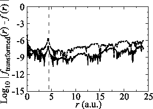
In Fig. 6, the numerical error accompanied
by the present method in two consecutive transforms of the
PAO functions of the oxygen
, the
function should recover the original shape by two consecutive
transforms and thus we can illustrate the numerical error by
comparing the input function and the back-and-forth transformed
function.
In Fig. 6, the numerical error accompanied
by the present method in two consecutive transforms of the
PAO functions of the oxygen  and
and  states is plotted.
The parameters used for the calculations are:
states is plotted.
The parameters used for the calculations are:  and
and
 .
The error is less than
.
The error is less than  which may not be sufficiently
small but is acceptable in practice depending on the particular
problems.
which may not be sufficiently
small but is acceptable in practice depending on the particular
problems.
Figure 5:
(a) PAO functions of the oxygen  (solid line) and
  (dashed line) states, where the confinement length is
 (indicated by the vertical dashed line).
(b) Transformed PAO functions of the oxygen
(indicated by the vertical dashed line).
(b) Transformed PAO functions of the oxygen  (solid line) and
  (dashed line) states.
|
Figure 6:
Numerical error accompanied by the back-and-forth transform of the PAO functions of the oxygen  (solid line) and
  (dashed line) states.
|
Figure 7:
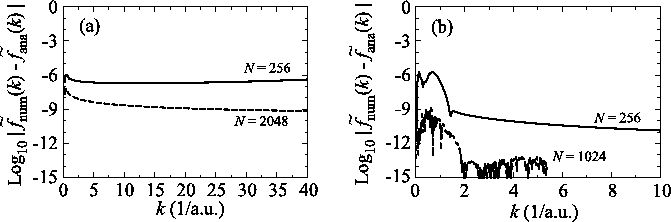
Numerical error accompanied by the Siegman-Talman method in performing
the back-and-forth transform of the PAO function of the oxygen  state.
The calculations are performed with various
state.
The calculations are performed with various  , namely,
128 (solid line), 1024 (dashed line), and 2048 (dash-dotted line),
while keeping
, namely,
128 (solid line), 1024 (dashed line), and 2048 (dash-dotted line),
while keeping
 and
and
 .
.
|
For the purpose of comparison, we have performed the
back-and-forth transform of the PAO function of the oxygen  state with the method proposed by Siegman and Talman [9,10].
In the calculations, we have used
state with the method proposed by Siegman and Talman [9,10].
In the calculations, we have used
 and
and
 .
As shown in Fig. 7, to suppress the error
less than
.
As shown in Fig. 7, to suppress the error
less than  in the region
  ,
a very large number of quadrature points (
,
a very large number of quadrature points ( ) are required.
As in this case, due to the use of the linear coordinate grid,
a small number of the grid points is enough for the present method
to achieve the same degree of accuracy.
The computation time has also been measured by taking the average
of the cpu time used for 1000 repetitions of a set of transforms, which
was carried out on a machine with an Intel Core i7 processor at 2.67 GHz.
The program code of the Siegman-Talman method is also implemented
by the authors according to the article [10].
The Siegman-Talman method costs 0.64 msec per transform with
) are required.
As in this case, due to the use of the linear coordinate grid,
a small number of the grid points is enough for the present method
to achieve the same degree of accuracy.
The computation time has also been measured by taking the average
of the cpu time used for 1000 repetitions of a set of transforms, which
was carried out on a machine with an Intel Core i7 processor at 2.67 GHz.
The program code of the Siegman-Talman method is also implemented
by the authors according to the article [10].
The Siegman-Talman method costs 0.64 msec per transform with
 , and the present method costs 1.32 msec per
transform with
, and the present method costs 1.32 msec per
transform with  .
In this measurement, each transform is performed independently so that
any speed-up technique is not used such as skipping redundant calculations and
reusing recources.
This is just a rough estimation, but looks reasonable considering
the theoretical computation cost of the both methods
(i.e. the computation cost for the Siegman-Talman method
is basically coming from that of two Fourier transforms, whereas
the present method requires three times of the Fourier transforms
as well as the additional numerical integrations).
In the present method, as mentioned before, once a transform with an order
is performed,
another transform with another order
can also be performed by repeating only the final step.
In the set of transform with 15 different orders for a single input function, a substantial
amount of redundant calculations are included. In fact, similar redundancy arises also in the
Siegman-Talman method. By skipping such redundant calculations, average time per transform
reduces to 0.45 msec for the Siegman-Talman method and to 0.22 msec for the present method,
in the same measurement as previous one except for the skipping. Therefore, the present method
can be quite effective for a particular type of applications where a single input function is
required to be transformed several times with different orders. An example of such applications
is the calculation of two-electron integrals in molecules and solids [4,5].
The authors believe that the present method is an alternative
to the Siegman-Talman method with comparable efficiency.
The most significant difference of the present method from the
Siegman-Talman method is the use of a uniform coordinate grid.
For many physical systems which are better described by the
uniform coordinate grid, a small number of the quadrature points
are required, which gives the advantages not only in the computation speed
but also in, for example, the reduction in the memory size and
communication traffic in parallelized computations.
.
In this measurement, each transform is performed independently so that
any speed-up technique is not used such as skipping redundant calculations and
reusing recources.
This is just a rough estimation, but looks reasonable considering
the theoretical computation cost of the both methods
(i.e. the computation cost for the Siegman-Talman method
is basically coming from that of two Fourier transforms, whereas
the present method requires three times of the Fourier transforms
as well as the additional numerical integrations).
In the present method, as mentioned before, once a transform with an order
is performed,
another transform with another order
can also be performed by repeating only the final step.
In the set of transform with 15 different orders for a single input function, a substantial
amount of redundant calculations are included. In fact, similar redundancy arises also in the
Siegman-Talman method. By skipping such redundant calculations, average time per transform
reduces to 0.45 msec for the Siegman-Talman method and to 0.22 msec for the present method,
in the same measurement as previous one except for the skipping. Therefore, the present method
can be quite effective for a particular type of applications where a single input function is
required to be transformed several times with different orders. An example of such applications
is the calculation of two-electron integrals in molecules and solids [4,5].
The authors believe that the present method is an alternative
to the Siegman-Talman method with comparable efficiency.
The most significant difference of the present method from the
Siegman-Talman method is the use of a uniform coordinate grid.
For many physical systems which are better described by the
uniform coordinate grid, a small number of the quadrature points
are required, which gives the advantages not only in the computation speed
but also in, for example, the reduction in the memory size and
communication traffic in parallelized computations.
Summary
In conclusion, we have proposed and demonstrated a new method
for the numerical evaluation of SBT.
Sufficiently accurate results are obtained in transforming
analytic atomic orbital functions.
Even the non-analytic PAO functions can be transformed
by the present method with a practically acceptable accuracy.
Application of the present method to evaluate the
electron-electron repulsion integrals is currently in progress
by the authors.
A similar framework could also be developed for the Hankel
transform of integer order, by using the integral expression
of the Bessel function in terms of the Gegenbauer polynomials.
Acknowledgments
This work was partly supported by CREST-JST and the
Next Generation Super Computing Project, Nanoscience Program,
MEXT, Japan.
For given values and derivatives of  at two points,
a polynomial which interpolates locally between the points can be obtained
by simply solving simultaneous equations.
For example, a cubic (
at two points,
a polynomial which interpolates locally between the points can be obtained
by simply solving simultaneous equations.
For example, a cubic ( ) polynomial which interpolates locally between
 and
and  is given by
 |
(A.1) |
where the coefficients are
A quintic ( ) polynomial is obtained by using the second
derivatives of
) polynomial is obtained by using the second
derivatives of  ,
,
 |
(A.6) |
where the coefficients are
 |
 |
(A.7) |
 |
 |
(A.8) |
 |
 |
(A.9) |
 |
 |
(A.10) |
 |
 |
(A.11) |
 |
 |
(A.12) |
The segment of integral  is evaluated in another way.
Since
is evaluated in another way.
Since  is usually very small, the Fourier cosine/sine
transform can be expanded in a Taylor's series.
If
is usually very small, the Fourier cosine/sine
transform can be expanded in a Taylor's series.
If  is even, the Fourier cosine transform becomes
where
 |
(B.5) |
Therefore, the segment for an even number of  is given as
Similarly, for an odd number of  , it is
 |
 |
(B.8) |
- [1]
L. W. Person, P. Benioff, Calculations for quasi-elastic scattering
 ,
,
 and
and
 at 460
 , Nucl. Phys. A187 (1972) 401.
- [2]
A. E. Glassgold, G. Ialongo, Angular distribution of the outgoing electrons in
electronic ionization, Phys. Rev. 175 (1968) 151.
- [3]
M. Liguori, A. Yadav, F. K. Hansen, E. Komatsu, S. Matarrese, B. Wandelt,
Temperature and polarization CMB maps from primordial non-Gaussiantities of
the local type, Phys. Rev. D 76 (2007) 105016.
- [4]
J. D. Talman, Numerical methods for multicenter integrals for numerically
defined basis functions applied in molecular calculations, Int. J. Quantum
Chem. 93 (2003) 72.
- [5]
M. Toyoda, T. Ozaki, Numerical evaluation of electron repulsion integrals for
pseudoatomic orbitals and their derivatives, J. Chem. Phys. 130 (2009)
124114.
- [6]
S. M. Candel, An algorithms for the Fourier Bessel transform, Comput. Phys. Comm.
23 (1981) 343.
- [7]
J. D. Secada, Numerical evaluation of the Hankel transform, Comput. Phys. Comm.
116 (1999) 278.
- [8]
V. K. Singh, Om P. Singh, R. K. Pandey, Numerical evaluation of the Hankel
transform by using linear Legendre multi-wavelets, Comput. Phys. Comm. 179
(2008) 424.
- [9]
A. E. Siegman, Quasi fast Hankel transform, Opt. Lett. 1 (1977) 13.
- [10]
J. D. Talman, Numerical Fourier and Bessel transforms in logarithmic variables,
J. Comput. Phys. 29 (1978) 35.
-
J. D. Talman, NumSBT: A subroutine for calculating spherical Bessel transforms
numericaly, Computer Phys. Comm. 180 (2009) 332.
- [12]
O. A. Sharafeddin, H. F. Bowen, D. J. Kouri, D. K. Hoffman, Numerical
evaluation of spherical Bessel transforms via fast Fourier transforms, J.
Comput. Phys. 100 (1992) 294.
- [13]
D. Lemoine, The discrete Bessel transform algorithm, J. Chem. Phys. 101 (1994)
3936.
- [14]
M. Abramowitz, I. A. Stegun (Eds.), Handbook of Mathematical Functions with
Formulas, Graphs, and Mathematical Tables, Dover publications, 1972.
- [15]
T. Ozaki, Variationally optimized atomic orbitals for large-scale electronic
structures, Phys. Rev. B 67 (2003) 155108.
This document was generated using the
LaTeX2HTML translator Version 2002-2-1 (1.71)
Copyright © 1993, 1994, 1995, 1996,
Nikos Drakos,
Computer Based Learning Unit, University of Leeds.
Copyright © 1997, 1998, 1999,
Ross Moore,
Mathematics Department, Macquarie University, Sydney.
TOYODA Masayuki
2009-09-30
![$\displaystyle \hspace{4em} \left. + \int_0^1 dt \ P_\ell(-t) \int_0^\infty dr \ e^{-ikrt} f(r) r^2 \right]$](img64.png)