Numerical Evaluation of Electron Repulsion Integrals for Pseudo-Atomic Orbitals and Their Derivatives

Masayuki Toyoda$^*$ and Taisuke Ozaki
Research Center for Integrated Science, Japan Advanced Institute of Science and Technology,
1-1, Asahidai, Nomi, Ishikawa 932-1292, Japan

Copyright 2009 American Institute of Physics. This article is provided by the author for the reader's personal use only. Any other use requires prior permission of the author and the American Institute of Physics. The following article appeared in Journal of Chemical Physics 130, 124114 (2009) and may be found at http://link.aip.org/link/?JCPSA6/130/124114/1.
 
NOTICE: This is the authorfs version of a work accepted for publication by American Institute of Physics. Changes resulting from the publishing process, including peer review, editing, corrections, structural formatting and other quality control mechanisms, may not be reflected in this document. Changes may have been made to this work since it was submitted for publication.

Abstract

A numerical method to calculate the four-center electron-repulsion integrals for strictly localized pseudo-atomic orbital basis sets has been developed. Compared to the conventional Gaussian expansion method, this method has an advantage in ease of combination with $O(N)$ density functional calculations. Additional mathematical derivations are also presented including the analytic derivatives of the integrals with respect to atomic positions and spatial damping of the Coulomb interaction due to the screening effect. In the numerical test for a simple molecule, the convergence up to $10^{-5}$ Hartree in energy is successfully obtained with a feasible cost of computation.

Introduction

In ab initio electronic structure calculations based on the density-functional theory (DFT), the Fock exchange for Kohn-Sham orbitals has been occasionally used as the ``exact'' exchange in order to improve the poor description of exchange energy by the Dirac exchange which is the standard functional used in the local density approximation (LDA) and the generalized gradient corrections (GGA). In recent years, various molecular systems have been calculated by using the hybrid functional methods [1], such as B3LYP [2,3] and PBE0 [4], where a certain amount of the Fock exchange is admixed with the LDA/GGA exchange-correlation functionals. The introduction of the non-local Fock exchange significantly improves the delocalization error [5] in the semi-local LDA/GGA functional and presents better thermochemical and structural properties of molecules.

The heavy computational demand to evaluate the Fock exchange is, however, a serious drawback. The studies for large molecules and solids are thus very limited. One solution for this problem is given in the Heyd-Scuseria-Ernzerhof (HSE) hybrid functional [6] where the long tail of the Coulomb interaction is somewhat artificially damped. The successful application of the HSE hybrid functional to extended systems, typified by the surprisingly accurate values of the band-gap energies of semiconductors [7], implies that the damping scheme they introduced is not just conducive to reducing the computational cost, but reasonable as well to describe the screening of the Coulomb interaction in real materials.

The Fock exchange consists of the four-center electron repulsion integrals (ERI) among basis functions. Since the integration can be performed analytically with the Gaussian-type orbital (GTO) basis functions, the Gaussian-expansion method is conventionally used in the evaluation of ERI where the basis functions are expanded in terms of GTO basis set [8,9,10]. However, the Gauss transform of a numerically defined function might require an indirect way such as a fitting process of the function to analytic functions unlike that for the Slater-type orbital (STO) functions [8]. While, in our method, ERI is evaluated directly from arbitrarily defined basis functions. Specifically in the $O(N)$ DFT calculation codes, such as CONQUEST [11], SIESTA [12] and OpenMX [13,14,15], the strictly localized pseudo-atomic orbital (PAO) basis sets are commonly used since the real space sparsity of the resultant Hamiltonian and overlap matrices enables us to combine the scheme with various $O(N)$ methods and to parallelize the computation by the domain decomposition in real space. Therefore, toward the implementation of the hybrid functionals or any other methods which utilizes the Fock exchange in the $O(N)$ DFT calculations, an effective numerical method is required to evaluate the Fock exchange with using the non-analytic PAO basis functions.

In this paper, we present a numerical procedure to calculate the four-center ERI for the numerically defined basis functions. We briefly review the mathematical derivations in the next section. Then, based on the formulations, we derive the analytic derivatives of the integrals with respect to atomic positions, which are required for the calculation of the forces on atoms. Our derivation is fully analytic and consistent with the integrals themselves. We also derive the formulation of ERI when the spatial damping of the Coulomb interaction is introduced as in the HSE hybrid functional.

Formulation

Numerical evaluation of ERI

The essential mathematical analysis described in this section is provided by Talman [16]. The considered wavefunctions are expressed as the linear combination of the PAO basis functions (LCPAO) and each basis function is a product of a numerically defined radial function $f(r)$ and an eigenfunction of angular momentum i.e. the spherical harmonic function $Y_L({\hat r})$ for given angular momentum $L = (\ell, m)$:

$$\varphi(\vec r) = f(r) Y_{L}(\hat r) .$$ (1)

The Fock exchange for the wavefunctions is then expressed as the sum of ERI for the basis functions. In general, ERI for four basis functions centered at different positions $\vec a_1$, $\vec a_2$, $\vec a_3$ and $\vec a_4$ is defined as follows:

$$I_4 \equiv \iint \varphi_1^*(\vec r - \vec a_1) \varphi_2(\vec r ... ... \varphi_3(\vec r' - \vec a_3) \varphi_4^*(\vec r' - \vec a_4) \ d^3 r d^3 r' .$$ (2)

$I_4$ is also denoted as $(\varphi_1 \varphi_2\vert \varphi_3 \varphi_4)$ to make the order of the basis functions clear. This integral is quite difficult to compute since the integration has to be performed over six-dimensional space coordinates. To reduce the dimensionality of the coordinates, one first needs to describe the overlap of the basis functions $\varphi_1$ and $\varphi_2$ as a function centered at an arbitrarily chosen center $\vec c$ which will be referred to as the overlap function later, and, similarly, the overlap of $\varphi_3$ and $\varphi_4$ at another center $\vec c'$,

$$F^{12}(\vec r - \vec c) = \varphi_1(\vec r - \vec a_1) \varphi_2^*(\vec r - \vec a_2) ,$$ (3)

$$F^{34}(\vec r - \vec c') = \varphi_3(\vec r - \vec a_3) \varphi_4^*(\vec r - \vec a_4) .$$ (4)

Then, the integral Eq. (2) becomes

$$I_4 = \iint \left( F^{12}(\vec r - \vec c) \right)^* \frac{1}{\vert \vec r - \vec r' \vert} F^{34}(\vec r'- \vec c') \ d^3 r d^3 r' .$$ (5)

By using the Fourier transform of the Coulomb interaction $1/r$,

$$\int \frac{e^{i \vec k \cdot \vec r}}{r} \ d^3 r = \frac{4 \pi}{k^2} ,$$ (6)

the integral in reciprocal space is expressed as a single-center integral,

$$I_4 = \frac{1}{2 \pi^2} \int \frac{1}{k^2} \left( {\tilde F}^{12}(\vec k) \right)^* {\tilde F}^{34}(\vec k) e^{i \vec k \cdot \vec R} \ d^3 k ,$$ (7)

where $\vec R \equiv \vec c' - \vec c$ and ${\tilde F}^{ij}$ are the Fourier transformed functions of Eqs. (3) and (4). Since ${\tilde F}^{ij}$ are also expanded in terms of the spherical harmonic functions,

$${\tilde F}^{ij}(\vec k) = 4 \pi \sum_L i^{\ell} {\tilde P}^{ij}_L(k) Y_L(\hat k) ,$$ (8)

the angular part of the integral in Eq. (7) can be performed analytically, where the overlap coefficient, ${\tilde P}^{ij}_L(k)$, is a radial function of $k$ which will be discussed later on. Finally, the integral Eq. (2) is broken down to a sum of single-dimensional integrals as follows:

$$I_4 = 32 \pi \sum_L \sum_{L'} \sum_{\Lambda = (\lambda, \mu)} i^{... ...mbda} G^L_{L' \Lambda} Q^\lambda_{L L'}(R) \left( Y_\Lambda(\hat R) \right)^* ,$$ (9)

$$Q^\lambda_{L L'}(R) \equiv \int_0^\infty j_\lambda(kR) \left( {\tilde P}^{12}_L(k) \right)^* {\tilde P}^{34}_L(k) \ dk ,$$ (10)

where $G^L_{L' \Lambda}$ is the Gaunt coefficients defined by

$$G^{L}_{L' \Lambda} \equiv \int \left( Y_L(\hat r) \vphantom{\sum} \right)^* Y_{L'}(\hat r) Y_{\Lambda}(\hat r) \ d \Omega_r .$$ (11)

The remaining problem is how to calculate the overlap coefficients ${\tilde P}_L^{ij}$ in Eq. (8). In order to calculate them, the translation of expansion center of a basis function is considered based on the investigation by Löwdin [17] as follows:

$$\varphi_i(\vec r - \vec a) = \sum_\Lambda \alpha_\Lambda^i(r, \vec a) Y_\Lambda(\hat r) .$$ (12)

The coefficients $\alpha^i_\Lambda$, often referred to as $\alpha$-function, are given by

$$\alpha^i_\Lambda(r, \vec a) = 4 \pi \sum_{\Lambda'} i^{\ell_i - \... ...{L_i}_{\Lambda \Lambda'} \Gamma^i_{\lambda \lambda'}(r, a) Y_{\Lambda'}(\hat a)$$ (13)

with a function of $r$ and $\vec a$ defined by

$$\Gamma^i_{\lambda \lambda'}(r, a) = \frac{2}{\pi} {\cal S}^{(\lambda)} \left[ \vphantom{\sum} j_{\lambda'}(ka) {\tilde f}_i(k) \right] .$$ (14)

Here, ${\cal S}^{(\ell)}$ is the $\ell$-th order spherical Bessel transform and ${\tilde f}_i(k)$ is the transformed radial function given by

$${\tilde f}_\ell(k) = {\cal S}^{(\ell_i)} \left[ \vphantom{\sum} f_i(r) \right] \equiv \int_0^\infty j_{\ell_i}(kr) f_i(r) r^2 \ dr .$$ (15)

The overlap functions, Eqs. (3) and (4), are described in terms of $\alpha$-functions Eq. (13):

$$F^{ij}(\vec r) = \varphi_i(\vec r - (\vec a_1 - \vec c)) \varphi_j^*(\vec r - (\vec a_2 - \vec c))$$

$$= \sum_L P^{ij}_L(r, \vec a_i - \vec c, \vec a_j - \vec c) Y_L(\hat r) ,$$ (16)

where

$$P^{ij}_L(r, \vec a_i - \vec c, \vec a_j - \vec c) = \sum_\Lambda ... ...ec a_i - \vec c) \left( \alpha^{j}_{\Lambda'}(r, \vec a_j - \vec c) \right)^* .$$ (17)

Finally, by transforming Eq. (17), the overlap coefficients in reciprocal space are obtained as

$${\tilde P}^{ij}_L(k) = {\cal S}^{(\ell)} \left[ \vphantom{\sum} P^{ij}_L(r, \vec a_i - \vec c, \vec a_j - \vec c) \right] .$$ (18)

Let us summarize how to compute ERI in the present approach: The first step is to transform the radial part of the basis functions by Eq. (15). Then, for every pair of orbitals, $\alpha$-functions are calculated through Eqs. (13) and (14). From those $\alpha$-functions, the overlap coefficients Eq. (17) and the transformed ones Eq. (18) are obtained. Finally, the integral Eq. (9) is calculated by summing up the radial integrals Eq. (10).

Fast Spherical Bessel transform

In the above approach, the spherical Bessel transform (SBT) is performed at three different places, namely, Eqs. (14), (15) and (18). Since the orders of the transforms are different and high at each step, this process can be a source of numerical errors as well as a bottleneck in the computation speed. A careful examination is therefore required in implementing the numerical method of SBT.

In the preceding works by Talman, the fast spherical Bessel transform technique is used, which is proposed by Siegman [18] and Talman [19]. In our experience of testing several numerical techniques, such as the discrete Bessel transform [20] and the asymptotic expansion method [21], we have reached the conclusion that the Siegman-Talman's fast SBT method is actually the most stable and fast for the present approach [22]. It, however, still suffers from oscillating numerical error in high-order transforms. The error becomes more significant for the PAO basis functions than the analytic basis functions because of their finite truncation. Fortunately, the oscillating error can be substantially suppressed by applying a simple correction to the fast SBT method as we describe later in this section.

In the fast SBT method, the radial variables $r$ and $k$ are changed to their logarithms,

$$\rho = \ln (r) , \quad \kappa = \ln(k) .$$ (19)

Then SBT of a function $f(r)$ with order $\ell$,

$${\tilde f}(k) = {\cal S}^{(\ell)} \left[ \vphantom{\sum} f(r) \right] \equiv \int_0^\infty j_\ell(kr) f(r) r^2 \ dr ,$$ (20)

becomes a convolution-type integral as follows:

$${\tilde f}(k) = {\tilde f}(e^\kappa)$$

$$= e^{(m-3/2) \kappa} \hphantom{=} \times {\cal F}\left[ M_{\ell,m}(t) \ {\cal F}\left[ e^{(m+3/2)\rho} f(e^\rho) \right] \right] ,$$ (21)

where $m = 0, 1, 2, \cdots \ell$ is an arbitrarily chosen parameter and ${\cal F}$ is the Fourier transform.

The function $M_{\ell,m}(t)$ is the Fourier transformed spherical Bessel function:

$$M_{\ell, m}(t) = \frac{1}{2\pi} \int_{-\infty}^\infty e^{-i t\rho} e^{(3/2-m)\rho} j_\ell(e^\rho) \ d\rho ,$$ (22)

where the integral can be performed analytically [19]. The transform, Eq. (21), is thus reduced to a couple of consecutive one-dimensional Fourier transforms, where we can take advantages of the speed of the fast Fourier transform (FFT) algorithm.

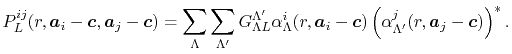
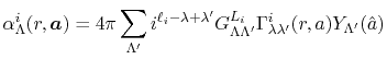
As mentioned before, the fast SBT method suffers from the oscillating numerical error in high-order transforms. In Fig. 1, a typical example of such error is shown, where a PAO basis function is transformed with the order $\ell = 14$ and $m = 0$, and then back-transformed with the same order. In the transformed function (the upper middle panel), the oscillating error appears in the small-$k$ region. After the back-and-forth transform (the upper right-hand panel), the accumulation of error is observed. Often, the error approaches quickly to infinity and the computation crashes.

In order to avoid the error, a simple correction is applied. Since the error appears only in the small-$k$ region, we perform the integration of Eq. (20) for some selected $k$-points between 0 and $k_0$ by using the straightforward trapezoidal method, where $k_0$ is smaller than the smallest $k$-points used in the final integration Eq. (10) so that the effect of the correction can be negligible, but the numerical breakdown can be avoided. By a linear interpolation between the selected $k$-points, we obtain another transformed function ${\tilde g}(k)$, in addition to ${\tilde f}(k)$. Then we replace ${\tilde f}(k)$ with ${\tilde g}(k)$ for $k < k_0$ as follows:

$${\tilde f}^\mathrm{corrected}(k) = {\tilde f}(k)\Theta(k - k_0) + {\tilde g}(k) \Theta(k_0 - k) .$$ (23)

This rather crude way of correction actually serves for the practical purpose. The lower panels of Fig. 1 show the example of the back-and-forth transform of the PAO basis function with the corrected fast SBT. Here, we use $k_0 = 10^{-2}$ and the straightforward integration are performed only for three selected $k$-points which are $k_0$, $10^{-4}$ and 0. It is confirmed that the oscillating error is successfully suppressed.

Figure 1: Accumulation of numerical error by back-and-forth transforms with the fast SBT method. The input function (a) is a PAO orbital of H atom for $\ell=2$ and $n_\mathrm{node}=4$. The transformed function of (a) is plotted in the panel (b), and the back-transformed of (b) in the panel (c). In the lower panels (d), (e) and (f), accumulation of numerical error by back-and-forth transforms with our modified fast SBT method is shown, where the error is substantially suppressed.

Derivatives

For the calculation of forces acting on atoms, we derive the derivatives of the integral Eq. (9) with respect to atomic positions. In our derivation, the expansion centers for the overlap functions are assumed to be given by the following forms:

$$\vec c = p \ \vec a_1 + (1-p) \ \vec a_2 ,$$ (24)

$$\vec c' = p' \ \vec a_3 + (1-p') \ \vec a_4 ,$$ (25)

where $0 \le p (p') \le 1$. Having in mind that $\vec R = \vec c' - \vec c$, the derivatives are obtained as

$${\vec\nabla}_{\vec a_1} I_4 = 32 \pi \sum_{L L' \Lambda} i^{\ell'-\ell+\lambda} G^\Lambda_{L L'} \left( \vphantom{\sum} -p {\vec A} + {\vec B}_{12} \right) ,$$ (26)

$${\vec\nabla}_{\vec a_2} I_4 = 32 \pi \sum_{L L' \Lambda} i^{\ell'-\ell+\lambda} G^\Lambda_{L L'} \left( \vphantom{\sum} -(1-p) {\vec A} - {\vec B}_{12} \right) ,$$ (27)

$${\vec\nabla}_{\vec a_3} I_4 = 32 \pi \sum_{L L' \Lambda} i^{\ell'-\ell+\lambda} G^\Lambda_{L L'} \left( \vphantom{\sum} p' {\vec A} + {\vec B}_{34} \right) ,$$ (28)

$${\vec\nabla}_{\vec a_4} I_4 = 32 \pi \sum_{L L' \Lambda} i^{\ell'-\ell+\lambda} G^\Lambda_{L L'} \left( \vphantom{\sum} (1-p') {\vec A} - {\vec B}_{34} \right) ,$$ (29)

where the vectors $\vec A$, $\vec B_{12}$ and $\vec B_{34}$ are defined as

$${\vec A} \equiv A \ Y_{\Lambda}(\hat R) \ {\vec e}_R + Q^\lambda_... ...eta} \frac{\partial Y_\Lambda(\hat R)}{\partial \phi} \ {\vec e}_\phi \right) ,$$ (30)

$$A \equiv \int_0^\infty k \left( \frac{d}{dz} j_\lambda(z) \right)_{z=kR} {\tilde P}^{12}_{L}(k) {\tilde P}^{34}_{L'}(k) \ dk ,$$ (31)

$${\vec B}_{12} \equiv \int_0^\infty j_\lambda(kR) \left( \vphantom{\sum} {\vec\nabla}_{\vec a_1} {\tilde P}^{12}_L(k) \right) {\tilde P}^{34}_{L'}(k) \ dk ,$$ (32)

$${\vec B}_{34} \equiv \int_0^\infty j_\lambda(kR) {\tilde P}^{12}_L(k) \left( \vphantom{\sum} {\vec\nabla}_{\vec a_3} {\tilde P}^{34}_{L'}(k) \right) \ dk .$$ (33)

Here, the unit vectors are defined as follows:

$${\vec e}_R \equiv ( \sin \theta \cos \phi, \sin \theta \sin \phi, \cos \theta) ,$$ (34)

$${\vec e}_\theta \equiv ( \cos \theta \cos \phi, \cos \theta \sin \phi, -\sin \theta) ,$$ (35)

$${\vec e}_\phi \equiv (\sin \phi, \cos \phi, 0) ,$$ (36)

where $\theta$ and $\phi$ are the spherical coordinate components of the vector $\vec R$.

The vector $\vec A$ can be calculated immediately since all the differentiations in Eqs. (30) and (31) are taken for the analytic functions. As shown in the appendix, the differentiations of the overlap functions in Eqs. (32) and (33) can also be performed completely analytically. Note that the differentiations are taken only for $\vec a_1$ and $\vec a_3$ because the others can also be obtained via the following sum rule:

$${\vec\nabla}_{\vec a_1} {\tilde P}^{12}_L(k) + {\vec\nabla}_{\vec a_2} {\tilde P}^{12}_L(k) = 0 ,$$ (37)

$${\vec\nabla}_{\vec a_3} {\tilde P}^{34}_L(k) + {\vec\nabla}_{\vec a_4} {\tilde P}^{34}_L(k) = 0 .$$ (38)

The rule arises due to the assumption of Eqs. (24) and (25), and this is the reason why we have assumed them. There is another sum rule:

$${\vec\nabla}_{\vec a_1} I_4 + {\vec\nabla}_{\vec a_2} I_4 + {\vec\nabla}_{\vec a_3} I_4 + {\vec\nabla}_{\vec a_4} I_4 = 0 ,$$ (39)

which is a more general one arising from the definition of the integral. It is easily confirmed that the derivatives Eqs. (26), (27), (28) and (29) satisfy the rule.

Screening of the Coulomb interaction

We also derive the formulation of ERI when the screening of Coulomb interaction is introduced. The screening scheme is assumed to be the same with that used in the HSE hybrid functional [6],

$$\frac{1}{r} \to \frac{1 - \mathrm{erf}(\omega r)}{r} ,$$ (40)

where $\mathrm{erf}(\omega r)$ is the Gauss error function and $\omega$ is a screening parameter. The Fourier transform of the screened Coulomb interaction is

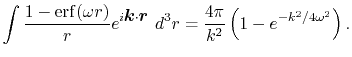$$\int \frac{1 - \mathrm{erf}(\omega r)}{r} e^{i \vec k \cdot \vec ... ...= \frac{4 \pi}{k^2} \left( \vphantom{\sum} 1 - e^{- k^2 / 4 \omega^2} \right) .$$ (41)

Therefore, the radial integral Eq. (10) becomes

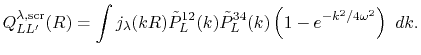$$Q^{\lambda, \mathrm{scr}}_{L L'}(R) = \int j_\lambda(kR) {\tilde ... ...e P}^{34}_L(k) \left( \vphantom{\sum} 1 - e^{- k^2 / 4 \omega^2} \right) \ dk .$$ (42)

Since the screening factor is independent of the atomic positions, the derivatives are still in the similar forms as Eqs. (26), (27), (28) and (29). Except, the radial integrals Eqs. (31), (32) and (33) are replaced with the screened ones as follows:

$$A^\mathrm{scr}(\omega) \equiv \int_0^\infty k \left( \frac{d}{dz}... ...2}_{L}(k) {\tilde F}^{34}_{L'}(k) \left( 1 - e^{-k^2/4 \omega^2} \right) \ dk ,$$ (43)

$${\vec B}_{12}^\mathrm{scr}(\omega) \equiv j\int_0^\infty j_\lambda(kR) \left( \vphantom{\sum} {\vec\... ...(k) \right) {\tilde F}^{34}_{L'}(k) \left( 1 - e^{-k^2/4 \omega} \right) \ dk ,$$ (44)

$${\vec B}_{34}^\mathrm{scr}(\omega) \equiv \int_0^\infty j_\lambda(kR) {\tilde F}^{12}_L(k) \left( \v... ...} {\tilde F}^{34}_{L'}(k) \right) \left( 1 - e^{-k^2/4 \omega^2} \right) \ dk .$$ (45)

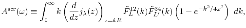
Computation speed

Our motivation is in the application of the Fock exchange in large systems such as large molecules and solids. In those systems, an enormous (infinite for solids) number of combinations of basis functions have to be considered. Fortunately for the PAO basis sets, since they are strictly confined in real space, the overlaps are exactly zero whenever the distance between the basis functions is longer than the sum of the confinement lengths. On the other hand, however, any two overlap functions can interact with each other even if they are separated quite far apart because of the infinitely long tail of the Coulomb interaction. By using the screening scheme described in the previous section, it might be justified to neglect the contribution from the far-separated pairs. Nevertheless, still a large number of pairs have to be calculated since the typical value of the screening parameter is $\omega = 0.15 a^{-1}$ and thus the effective screening length is $\sim 10 \AA$ [7]. Therefore, we should consider to make the computation faster for the final integration Eqs. (9) and (10). As already pointed out by Talman, the convergence of the summation Eq. (9) is very fast so that the cutoff angular momentum $\ell_\mathrm{max}$ and the number of $k$-sampling points $N_k$ can be decreased. We shall define new parameters ${\bar \ell}_\mathrm{max}$ and ${\bar N}_k$ for Eqs. (9) and (10) in order to distinguish from the original parameters $\ell_\mathrm{max}$ and $N_k$ which are used in the other parts. Typically, $\ell_\mathrm{max}$ has to be as large as $\sim 15$ to describe the overlap functions accurately. While, as shown later, ${\bar \ell}_\mathrm{max} = 6$ is enough to obtain $10^{-5}$ Hartree accuracy in energy even when $d$ orbitals are involved. Similarly, $N_k$ is required to be $\sim 1000$, while, in the final integration, the Gauss-Laguerre quadrature can be used which gives good convergence with ${\bar N}_k \sim 50$.

The location of the expansion centers $\vec c$ has also a significant effect on the convergence speed. In general, $\vec c$ is an orbital-dependent value. Therefore, since $\alpha$-functions Eqs. (13) and (14) depend on $\vec c$ (note that what we actually need is the terms in the right-hand side of Eq. (17)), one needs to calculate those coefficients of which the number is equivalent to that of neighboring orbitals. Here, we offer a suggestion that the computation cost may be reduced by choosing $\vec c$ at the middle of the two orbital centers,

$$\vec c = \frac{\vec a_1 + \vec a_2}{2} .$$ (46)

In this case, the required number of $\alpha$-functions is decreased by a factor of the number of orbitals per atom, which is typically $\sim 10$. Note that Eq. (46) is not the best choice if just one ERI is considered. In fact, the choice of of $\vec c$ with considering the spatial extent of each orbital gives faster convergence in the final integration [23]. Therefore, it becomes a competition between the convergence speed in performing a single integral and the required number of $\alpha$-functions.

Computation results

In order to check the convergence properties of our routine, we first performed calculations of ERI for a GTO basis set. Three different integrals $(ss\vert ss)$, $(ps\vert sp)$ and $(dd\vert dd)$ are calculated. The definition of the basis functions for the integrals is listed in Table 1. For all the integrals, the orbital locations are fixed to the corners of a square on the $x-y$ plane with edge length of 1; $\vec a_1 = ( 1/2, 1/2, 0)$, $\vec a_2 = ( 1/2, -1/2, 0)$, $\vec a_3 = (-1/2, 1/2, 0)$ and $\vec a_4 = (-1/2, -1/2, 0)$. The cutoff for the angular momentum is $\ell_\mathrm{max} = 15$ and the number of radial mesh points is $N = 1024$. In the final integration, the Gauss-Laguerre quadrature is used where the number of k-sampling points is ${\bar N}_k = 60$ and the summation is taken up to a reduced cutoff ${\bar \ell}_\mathrm{max}$. In Table 2, the calculated values of the integrals are shown for increasing ${\bar \ell}_\mathrm{max}$, where they are left blank after the convergence up to $10^{-5}$ Hartree is achieved. The exact values are also shown for comparison, which are obtained by using the analysis given in literature [9]. It is clearly found that the convergence becomes slower for orbitals with higher angular momentum. Nevertheless, the accurate values for all the integrals up to $10^{-5}$ Hartree are obtained with ${\bar \ell}_\mathrm{max} = 6$.

Table: Definition of the integrals in the calculations of ERI for GTO.

integral	function	radial	angular
$(ss\vert ss)$	$\varphi_1$, $\varphi_2$, $\varphi_3$, $\varphi_4$	$e^{-r}$	$Y^0_0$	$= 1/\sqrt{4 \pi}$
$(ps\vert sp)$	$\varphi_2$, $\varphi_3$	$e^{-r^2}$	$Y_0^0$	$= 1/\sqrt{4 \pi}$
	$\varphi_1$	$r e^{-r^2}$	$Y_1^{-1}$	$= \sqrt{3/8 \pi}(x-iy)/r$
	$\varphi_4$	$r e^{-r^2}$	$Y_1^1$	$= -\sqrt{3/8 \pi}(x+iy)/r$
$(dd\vert dd)$	$\varphi_1$	$r^2 e^{-r^2/2}$	$Y_2^{2}$	$= \sqrt{15/32\pi}(x^2-y^2+2ixy)/r^2$
	$\varphi_2$	$r^2 e^{-r^2/2}$	$Y_2^{-1}$	$= \sqrt{15/8\pi}(xz-iyz)/r^2$
	$\varphi_3$	$r^2 e^{-r^2/2}$	$Y_2^{1}$	$= -\sqrt{15/8\pi}(xz+iyz)/r^2$
	$\varphi_4$	$r^2 e^{-r^2/2}$	$Y_2^{-2}$	$= \sqrt{15/32\pi}(x^2-y^2-2ixy)/r^2$

Table: Convergence of the calculations of ERI for GTO basis set with respect to the cutoff parameter ${\bar \ell}_\mathrm{max}$.

	Integrals (Hartree)
${\bar \ell}_\mathrm{max}$	$(ss\vert ss)$	$(ps\vert sp)$	$(dd\vert dd)$
0	0.007608	0.002853	0.000000
1		0.002384	0.001055
2		0.002512	0.000305
3			0.002656
4			-0.001909
5			-0.001909
6			-0.001965
exact	0.007608	0.002512	-0.001966

As a more realistic example, we performed calculations of ERI of a methane molecule for a Slater-type orbital (STO) basis set. The basis functions and the atomic positions are summarized in Table 3. Our results and the comparison values which are calculated by using the Gaussian expansion method [9] are shown in Table 4. For all the integrals considered, ours and the comparison values agree with each other up to $10^{-5}$ Hartree. The difference from the comparison values is large for $(c1\vert c2)$ and $(cc\vert 12)$ because the C-$1s$ inner-shell orbital is involved. In general, the small spatial extent of such the inner-shell orbitals makes the convergence slower. This, however, would not have to be considered so seriously in the actual calculations if the contribution of the inner-shell electrons are included in the pseudopotentials.

Table: Basis functions and atomic positions in the calculations of methane molecule. The STO basis functions are normalized.

Symbol	Atom	Orbital	Position			Exponent
			$x$	$y$	$z$
$1$	H	$1s$	0	0	$-2$	$1.000$
$2$	H	$1s$	$4\sqrt{2}/3$	0	$2/3$	$1.000$
$3$	H	$1s$	$-2\sqrt{2}/3$	$2\sqrt{6}/3$	$2/3$	$1.000$
$4$	H	$1s$	$-2\sqrt{2}/3$	$-2\sqrt{6}/3$	$2/3$	$1.000$
$c$	C	$1s$	0	0	0	$5.700$
$x$	C	$2p_x$	0	0	0	$1.625$
$z$	C	$2p_y$	0	0	0	$1.625$

Table: Convergence of the calculations of ERI of methane molecule for the STO basis set. The symbols $1$, $2$, $3$, $4$, $c$, $x$ and $z$ specify the STO basis functions of H and C atoms. See Table 3 for details. The comparison values are taken from ref. [9].

	Integrals (Hartree)
${\bar \ell}_\mathrm{max}$	$(12\vert 34)$	$(12\vert 13)$	$(11\vert 23)$	$(c1\vert 34)$	$(c1\vert c2)$	$(cc\vert 12)$	$(c1\vert x2)$	$(c1\vert z2)$
0	0.031420	0.035743	0.097301	0.013109	0.011258	0.170321	0.026924	0.009519
1	0.031420	0.035743	0.097301	0.013010	0.011186	0.170321	0.020083	0.006288
2	0.030647	0.035666	0.095631	0.012719	0.011188	0.166242	0.020144	0.006106
3	0.030647	0.035666	0.095631	0.012723	0.011188	0.166242	0.019819	0.005914
4	0.030684	0.035694	0.095709	0.012743	0.011188	0.166578	0.019834	0.005902
5	0.030684	0.035694	0.095709	0.012743	0.011188	0.166578	0.019809	0.005887
6	0.030681	0.035694	0.095703	0.012741	0.011188	0.166531	0.019811	0.005887
comp.	0.030683	0.035694	0.095706	0.012741	0.011195	0.166536	0.019809	0.005885

Calculations of ERI for a PAO basis set are performed for the methane structure. The PAO data is taken from those used in OpenMX DFT calculation package [24]. The ground state orbitals generated by the confinement scheme [13] with the radius of 5.0 Bohr are used as the PAO basis functions for both the hydrogen and carbon atoms. The calculated values are shown in Table 5 where the parameters $\ell_\mathrm{max} = 15$, $N = 1024$ and ${\bar N}_k = 60$ are used. The comparison values are also calculated by using the present method with the enhanced parameters $\ell_\mathrm{max} = 20$ and $N = 4096$. As well as the analytic functions such as GTO and STO basis sets, even for the strictly localized PAO basis set, it is confirmed that the convergence up to $10^{-5}$ Hartree is obtained with ${\bar \ell}_\mathrm{max} = 6$.

Table: Convergence of the calculations of ERI of methane molecule for the PAO basis set. The symbols and the atomic positions are the same as in Table 3. The comparison values are also calculated by using the present method with enhanced parameters (see text for details).

	Integrals (Hartree)
${\bar \ell}_\mathrm{max}$	$(12\vert 34)$	$(12\vert 13)$	$(11\vert 23)$	$(c1\vert 34)$	$(c1\vert c2)$	$(cc\vert 12)$	$(c1\vert x2)$	$(c1\vert z2)$
0	0.031071	0.035881	0.096122	0.070962	0.158759	0.141194	-0.044336	0.047671
1	0.031071	0.035881	0.096122	0.071814	0.161936	0.141194	-0.030393	0.018107
2	0.030601	0.035835	0.095266	0.071497	0.162871	0.140576	-0.031044	0.020152
3	0.030601	0.035835	0.095266	0.071508	0.162823	0.140576	-0.030911	0.019802
4	0.030630	0.035860	0.095316	0.071517	0.162851	0.140577	-0.030915	0.019825
5	0.030630	0.035860	0.095316	0.071517	0.162851	0.140577	-0.030906	0.019826
6	0.030627	0.035860	0.095313	0.071516	0.162855	0.140577	-0.030905	0.019828
comp.	0.030630	0.035862	0.095318	0.071519	0.162859	0.140581	-0.030903	0.019829

The computation time in our method for calculating a single integral is 3.0 sec with Intel Xeon processor 3.2 GHz. This is too expensive compared to the time required in the conventional Gaussian-expansion method, e.g., one of the most sophisticated program takes only 0.5 - 1.3 msec per integral with Intel Pentium IV processor 3.2 GHz [10]. In our method, the most of the time is consumed in the calculation of the overlap functions. Fortunately, the required number of pairs is proportional to the number of the basis functions due to the finite truncation of the PAO basis functions, whereas the effort of the computation of ERIs scales quadratically as the number of the basis functions increases. In addition to that, the overlap functions can be reused for the calculations of ERI with a different pair of them, e.g., the overlap of 1 and 2 for $(12\vert 34)$ can also be used for $(12\vert 56)$ etc. Therefore, the computation efficiency in total can be significantly enhanced as the system size becomes larger.

Summary

In summary, a numerical method to evaluate ERI for the PAO basis sets has been developed. Based on the mathematical analysis by Talman, we derive the analytic derivatives and a spatial damping scheme for the Coulomb interaction. We also propose a numerical method for SBT of the strictly localized PAO basis functions, where the oscillating numerical error is well suppressed even for the high-order transforms. In the numerical calculations for a simple molecule, the convergence up to $10^{-5}$ Hartree in energy has been successfully obtained. The present method enables us to utilize state-of-the-art hybrid functional methods in the $O(N)$ DFT calculation programs.

Acknowledgments

This work was partly supported by CREST-JST and the Next Generation Super Computing Project, Nanoscience Program, MEXT, Japan.

addtoresetequationsection

Appendix

The derivatives of the overlap functions in the vectors Eqs. (32) and (33) are given as

$${\vec\nabla}_{\vec a_i} {\tilde P}^{ij}_L(k) = {\vec\nabla}_{\vec a_i} \mathrm{SBT}^{\ell} \left[ \vphantom{\sum} P_L(r, \vec a_i - \vec c, \vec a_j - \vec c; f_i, f_j) \right]$$

$$= \sum_{\Lambda \Lambda'} G^L_{\Lambda \Lambda'} \left\{ (1-p) \l... ...c u} \alpha^i_\Lambda(r, \vec u) \right) \alpha^j_{\Lambda'}(r, \vec v) \right.$$

$$\left. \hphantom{ \sum_{\Lambda \Lambda'} } - p \ \alpha^j_{\Lamb... ...right\}_{\substack{\vec u = \vec a_i - \vec c \\ \vec v = \vec a_j - \vec c}} ,$$ (A.1)

where we use the assumption in Eqs. (24) and (25). Then, the derivatives of the $\alpha$-functions are

$${\vec\nabla}_{\vec a} \alpha^L_\Lambda(r, a; f) = 4 \pi \sum_{\Lambda'} i^{\ell - \lambda + \lambda'} G^L_{\Lambd... ...\ell_{\lambda \lambda'}(r, a) \right) Y_{\Lambda'}(\hat a) \ {\vec e}_r \right.$$

$$\hspace{4em} + \frac{1}{a} \Gamma^\ell_{\lambda \lambda'}(r, a) \frac{\partial}{\partial \theta} Y_{\Lambda'}(\hat a) \ {\vec r}_\theta$$

$$\hspace{4em} \left. + \frac{1}{a \sin \theta} \Gamma^\ell_{\lambd... ...{\partial \phi} Y_{\Lambda'}(\hat a) \ {\vec e}_\phi \vphantom{\sum} \right\} ,$$ (A.2)

where the unit vectors are the similar to Eqs. (34), (35) and (36) where $\theta$ and $\phi$ are the spherical coordinate components of $\vec a$.

We come to the final equation, the derivatives of $\Gamma$ terms,

$$\frac{\partial}{\partial a} \Gamma^\ell_{\lambda \lambda'}(r, ) =... ...{dz} j_{\lambda'}(z) \right) \right\vert _{z = ka} {\tilde f}_\ell(k) \right] .$$ (A.3)

As derived here, all the components are derived analytically, without using any numerical differentiation.

In Eq. (30), there are terms proportional to $1/R$, which diverge as $R$ approaches to zero. In fact, $R$ can be a near-zero values when, for example, atoms are on a square lattice and the orbitals $\varphi_1$ and $\varphi_2$ are located at each end of a diagonal of the square, and $\varphi_3$ and $\varphi_4$ are at each end of the other diagonal. To avoid such numerical problem, we impose a lower limit on $R$ as follows:

$$R \to {\bar R} \equiv \sqrt{ R^2 + \delta^2 \exp( -R^2/\delta^2) } ,$$ (A.4)

where $\delta \ll 1$. The same problem may arise for the derivative of $\alpha$ terms (A2). However, we do not need to consider the case when $a$ is close to zero. This is because, in such case, the two orbitals are located on a same atom and thus the derivative of the overlap function (A1) should be always zero. Here, we assume that all the orbitals are located on the atoms. Note that the derivatives are not taken with respect to the orbital centers but to the atomic positions.

Bibliography

[1]  A. D. Becke, J. Chem. Phys. 98, 1372 (1993).

[2]  A. D. Becke, J. Chem. Phys. 98, 5648 (1993).

[3]  P. J. Stephens, F. J. Devlin, C. F. Chabalowski, and M. J. Frisch, J. Phys. Chem. 98, 11623 (1994).

[4]  C. Adamo and V. Barone, J. Chem. Phys. 110, 6158 (1999).

[5]  P. Mori-Sánchez, A. J. Cohen, and W. Yang, Phys. Rev. Lett. 100, 146401 (2008).

[6]  J. Heyd, G. E. Scuseria, and M. Ernzerhof, J. Chem. Phys. 118, 8207 (2003).

[7]  J. Heyd and G. E. Scuseria, J. Chem. Phys. 121, 1187 (2004).

[8]  I. Shavitt and M. Karplus, J. Chem. Phys. 36, 550 (1962).

[9]  H. Taketa, S. Huzinaga, and K. O-ohata, J. Phys. Soc. Jpn 21, 2313 (1966).

[10]  J. F. Rico, R. López, I. Ema, and G. Ramírez, J. Comp. Chem. 25, 1987 (2004).

[11]  A. S. Torralba et al., J. Phys.: Cond. Mat. 20, 294206 (2008).

[12]  J. M. Soler et al., J. Phys.: Cond. Mat. 14, 2745 (2002).

[13]  T. Ozaki and H. Kino, Phys. Rev. B 69, 195113 (2004).

[14]  T. Ozaki and H. Kino, Phys. Rev. B 72, 045121 (2005).

[15]  T. Ozaki, Phys. Rev. B 74, 245101 (2006).

[16]  J. D. Talman, Int. J. Quantum Chem. 93, 72 (2003).

[17]  P.-O. Löwdin, Adv. Phys. 5, 1 (1056).

[18]  A. E. Siegman, Opt. Lett. 1, 13 (1977).

[19]  J. D. Talman, J. Comput. Phys. 29, 35 (1978).

[20]  D. Lemoine, J. Chem. Phys. 101, 3936 (1994).

[21]  O. A. Sharafeddin, H. F. Bowen, D. J. Kouri, and D. K. Hoffman, J. Comput. Phys. 100, 294 (1992).

[22]  For example, in the discrete Bessel transform [20], an interpolation process is necessary because the sampling points vary for transforms of different orders. While, in the asymptotic expansion method [21], high-order trasnforms are quite unstable due to the factor inversely propotional to the $\ell$-th order of the variable where $\ell$ is the order of transform.

[23]  J. D. Talman, Int. J. Quantum Chem. 107, 1578 (2007).

[24]  http://www.openmx-square.org/.

About this document ...

This document was generated using the LaTeX2HTML translator Version 2002-2-1 (1.71)

Copyright © 1993, 1994, 1995, 1996, Nikos Drakos, Computer Based Learning Unit, University of Leeds.
Copyright © 1997, 1998, 1999, Ross Moore, Mathematics Department, Macquarie University, Sydney.