Total Energy and Forces: Ver. 1.2
Taisuke Ozaki, RCIS, JAIST
The OpenMX is based on density functional theories (DFT),
the norm-conserving pseudopotentials, and local pseudo-atomic
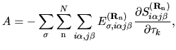
basis functions. The Kohn-Sham (KS) Bloch functions  are expanded
in a form of linear combination of pseudo-atomic basis functions (LCPAO)
are expanded
in a form of linear combination of pseudo-atomic basis functions (LCPAO)
 centered on site
  by
by
| |
|
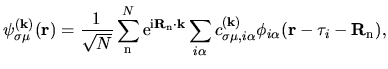 |
(1) |
where  and
and  are an expansion coefficient and pseudo-atomic
function,
are an expansion coefficient and pseudo-atomic
function,
 a lattice vector,
  a site index,
 spin index,
 an organized orbital
index with a multiplicity index
an organized orbital
index with a multiplicity index  , an angular momentum quantum number
  ,
and a magnetic quantum number
,
and a magnetic quantum number  .
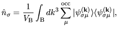
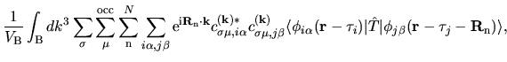
The charge density operator
.
The charge density operator
 for
the spin index
for
the spin index  is given by
| |
|
 |
(2) |
where  means the integration over the first
Brillouin zone of which volume is
means the integration over the first
Brillouin zone of which volume is  , and
, and
 means the summation over occupied states.
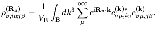
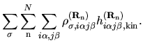
The charge density
means the summation over occupied states.
The charge density
 with the spin index
  is found as
with a density matrix defined by
| |
|
 |
(4) |
Although it is assumed that the electronic temperature
is zero in this notes, OpenMX uses the Fermi-Dirac function
with a finite temperature in the practical implementation.
Therefore, the force on atom becomes inaccurate for metallic
systems or very high temperature.
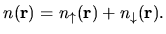
The total charge density  is the sum of
  and
and
 as follows:
| |
|
 |
(5) |
Also, it is convenient to define a difference charge density
 for later discussion as
where
 is an atomic charge density
evaluated by a confinement atomic calculations associated
with the site
is an atomic charge density
evaluated by a confinement atomic calculations associated
with the site  .
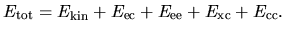
Within the local density approximation (LDA) and generalized
gradient approximation (GGA), the total energy of the collinear
case is given by the sum of
the kinetic energy
.
Within the local density approximation (LDA) and generalized
gradient approximation (GGA), the total energy of the collinear
case is given by the sum of
the kinetic energy  ,
the electron-core Coulomb energy
,
the electron-core Coulomb energy  ,
the electron-electron Coulomb energy
,
the electron-electron Coulomb energy  ,
the exchange-correlation energy
,
the exchange-correlation energy  ,
and the core-core Coulomb energy
,
and the core-core Coulomb energy  as
as
| |
|
 |
(7) |
The kinetic energy  is given by
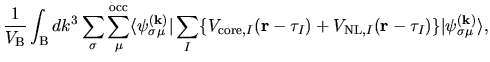
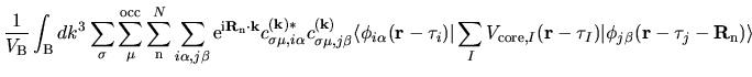
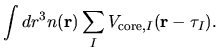
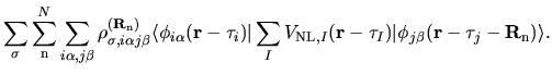
The electron-core Coulomb energy  is given by
two contributions
is given by
two contributions
 and
and
 related to the local and non-local parts of
pseudopotentials:
related to the local and non-local parts of
pseudopotentials:
where
 and
and
 are the local and
non-local parts of pseudopotential located on a site
are the local and
non-local parts of pseudopotential located on a site  .
Thus, we have
.
Thus, we have
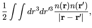
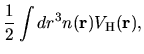
The electron-electron Coulomb energy  is given by
where  is decomposed into two contributions
 and
and
 coming from the superposition of
atomic charge densities and the difference charge density
coming from the superposition of
atomic charge densities and the difference charge density
 defined by
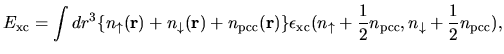
Within the LDA, the exchange-correlation energy  is given by
| |
|
 |
(15) |
where  is a charge density used for a partial core
correction (PCC).
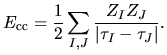
The core-core Coulomb energy
is a charge density used for a partial core
correction (PCC).
The core-core Coulomb energy  is given as repulsive
Coulomb interactions among effective core charge
is given as repulsive
Coulomb interactions among effective core charge  considered in the generation
of pseudopotentials by
considered in the generation
of pseudopotentials by
| |
|
 |
(16) |
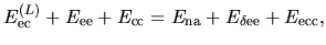
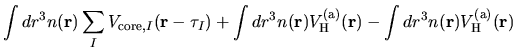
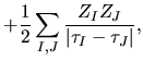
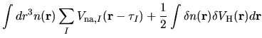
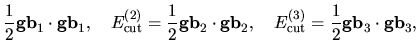
As discussed in the paper [1], for numerical accuracy
and efficiency it is important to reorganize the sum of
three terms
 ,
,  , and
, and  ,
as follows:
,
as follows:
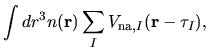
where
Therefore, we can reorganize these three terms as follows:
| |
|
 |
(19) |
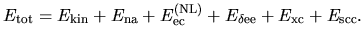
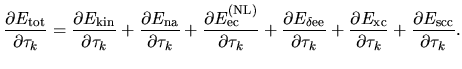
Following the reorganization of energy terms, the total energy
can be given by
| |
|
 |
(23) |
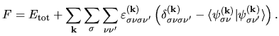
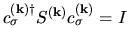
Considering the orthogonality relation among one-particle wave functions,
let us introduce a functional  with Lagrange's multipliers
 :
:
| |
|
 |
(24) |
The variation of the functional  with respect to the LCPAO
coefficients
with respect to the LCPAO
coefficients
 yields
the following matrix equation:
yields
the following matrix equation:
| |
|
 |
(25) |
Moreover, noting that the matrix
 for Lagrange's multipliers is Hermitian, and introducing
  diagonalizing
the matrix, we can transform above equation as:
diagonalizing
the matrix, we can transform above equation as:
| |
|
 |
(26) |
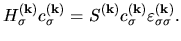
By renaming
 by
by
 ,
and defining the diagonal element of
,
and defining the diagonal element of
 to be
to be
 , we have a well known
Kohn-Sham equation in a matrix form as a generalized eigenvalue problem:
, we have a well known
Kohn-Sham equation in a matrix form as a generalized eigenvalue problem:
| |
|
 |
(27) |
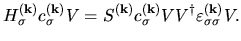
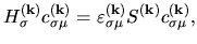
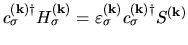
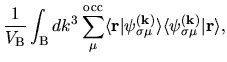
where the Hamiltonian and overlap matrices are given by
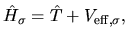
with a Kohn-Sham Hamiltonian operator
| |
|
 |
(30) |
and the effective potential
| |
|
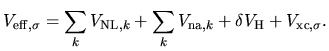 |
(31) |
The neutral atom potential
 is spherical
and defined within the finite range determined by
the cutoff radius
is spherical
and defined within the finite range determined by
the cutoff radius  of the confinement potential.
Therefore, the potential
of the confinement potential.
Therefore, the potential
 can be expressed
by a projector expansion as follows:
can be expressed
by a projector expansion as follows:
| |
|
 |
(32) |
where a set of radial functions
 is an orthonormal
set defined by a norm
is an orthonormal
set defined by a norm
 for radial
functions
for radial
functions  and
and  , and is calculated by the following Gram-Schmidt
orthogonalization [4]:
, and is calculated by the following Gram-Schmidt
orthogonalization [4]:
The radial function  used is pseudo wave
functions for both the ground and excited states under the same
confinement potential as used in the calculation of the atomic
electron density
used is pseudo wave
functions for both the ground and excited states under the same
confinement potential as used in the calculation of the atomic
electron density  [2,3].
The most important feature in the projector expansion is that the
deep neutral atom potential is expressed by a separable form,
and thereby we only have to evaluate the two-center integrals
to construct the matrix elements for the neutral atom potential.
As discussed later, the two-center integrals can be accurately
evaluated in momentum space. For details of the projector
expansion method, see also the reference [1].
The overlap integrals, matrix elements for the non-local potentials,
for the neutral atom potentials in a separable form discussed in
the Sec. 3, and for the kinetic operator consist of two-center integrals.
In this section, the evaluation of the two-center integrals is discussed.
The pseudo-atomic function
[2,3].
The most important feature in the projector expansion is that the
deep neutral atom potential is expressed by a separable form,
and thereby we only have to evaluate the two-center integrals
to construct the matrix elements for the neutral atom potential.
As discussed later, the two-center integrals can be accurately
evaluated in momentum space. For details of the projector
expansion method, see also the reference [1].
The overlap integrals, matrix elements for the non-local potentials,
for the neutral atom potentials in a separable form discussed in
the Sec. 3, and for the kinetic operator consist of two-center integrals.
In this section, the evaluation of the two-center integrals is discussed.
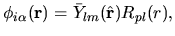
The pseudo-atomic function
 in Eq. (1) is given
by a product of a real spherical harmonic function
in Eq. (1) is given
by a product of a real spherical harmonic function  and a radial
wave function
and a radial
wave function  :
:
| |
|
 |
(35) |
where  means Euler angles,
  and
and  ,
for
,
for  , and
, and  radial coordinate.
Although the real function is used for the spherical harmonic function
in OpenMX instead of the complex function
radial coordinate.
Although the real function is used for the spherical harmonic function
in OpenMX instead of the complex function
 ,
firstly we consider the case with the complex function
,
firstly we consider the case with the complex function
 as
as
| |
|
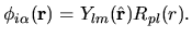 |
(36) |
After the evaluation of two-center integrals related to the complex function,
they are transformed into two-center integrals for the real function
 by matrix operations.
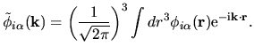
Then, the pseudo-atomic function
by matrix operations.
Then, the pseudo-atomic function
 given by Eq. (36)
can be Fourier-transformed as follows:
given by Eq. (36)
can be Fourier-transformed as follows:
| |
|
 |
(37) |
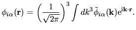
The back transformation is defined by
| |
|
 |
(38) |
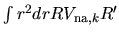
Noting the Rayleigh expansion
and putting Eqs. (36) and (40) into Eq. (37), we have
where we defined
| |
|
![$\displaystyle \tilde{R}_{pl}(k)=
\left[
\left( \frac{1}{\sqrt{2\pi}} \right )^3
4\pi
(-{\rm i})^{l}
\int dr
r^2
R_{pl}(r)
j_{L}(kr)
\right].$](img216.png) |
(42) |
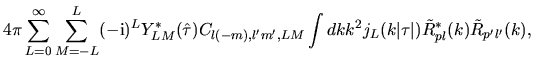
Using Eqs. (38), (40), and (41), the overlap integral is evaluated as follows:
where an integral in the third line was evaluated as
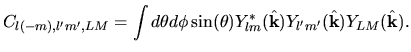
and one may notice Gaunt coefficients defined by
| |
|
 |
(45) |
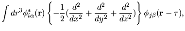
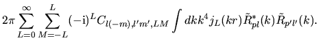
The matrix element for the kinetic operator can be easily found in the same
way as for the overlap integral as follows:
The two energy terms
 and
and  are discretized by a regular mesh
 in real space [5], while the integrations in
  ,
,
 ,
,  , and
, and
 can be reduced to two center integrals which can be
evaluated in momentum space.
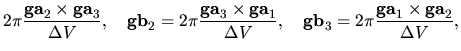
The regular mesh
can be reduced to two center integrals which can be
evaluated in momentum space.
The regular mesh
 in real space is
generated by dividing the unit cell with a same interval
which is characterized by
the cutoff energies
in real space is
generated by dividing the unit cell with a same interval
which is characterized by
the cutoff energies
 ,
,
 , and
, and
 :
:
where  ,
,  , and
, and  are
unit cell vectors of the whole system, and
are
unit cell vectors of the whole system, and  ,
,  , and
, and  are the number of division for
  ,
,  ,
and
,
and  -axes, respectively.
 ,
,  , and
, and  are determined so that the differences among
 ,
,
 , and
, and
 can be minimized starting from the given cutoff energy.
Using the regular mesh
can be minimized starting from the given cutoff energy.
Using the regular mesh
 ,
the Hartree energy
,
the Hartree energy
 associated with
the difference charge density
associated with
the difference charge density
 is discretized as
| |
|
 |
(51) |
The same regular mesh
 is also applied to
the solution of Poisson's equation to find
is also applied to
the solution of Poisson's equation to find
 .
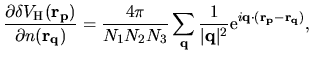
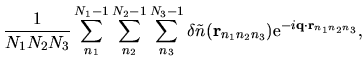
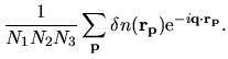
Then, the charge density is Fourier transformed by
.
Then, the charge density is Fourier transformed by
From
 , we can evaluate
 by
by
| |
|
 |
(53) |
Thus, we see that
 is also written
in a discretized form with the regular mesh as follows:
is also written
in a discretized form with the regular mesh as follows:
Within the LDA,  can be easily discretized
as well as
can be easily discretized
as well as
 by
by
For the GGA,  is discretized with the gradient of charge
density evaluated with a finite difference scheme in the same way in the LDA.
Since the derivative of the charge density
is discretized with the gradient of charge
density evaluated with a finite difference scheme in the same way in the LDA.
Since the derivative of the charge density  with respect to
 is given by
| |
|
 |
(56) |
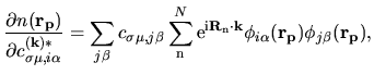
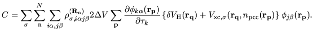
the matrix elements for
 and
and  in the
Kohn-Sham equation Eq. (27) are found by differentiating the
energies
in the
Kohn-Sham equation Eq. (27) are found by differentiating the
energies
 and
and  with respect to
 as follows:
and
where the quantities in the parenthesis ![$[]$](img321.png) correspond to the matrix elements.
correspond to the matrix elements.
| |
|
 |
(59) |
The derivative of the kinetic energy with respect to  is given by
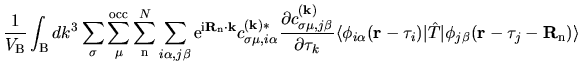
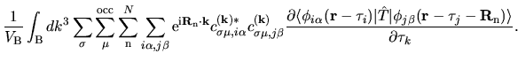
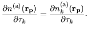
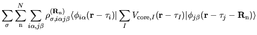
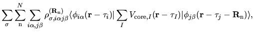
The derivative of the neutral atom potential energy with respect to
 is given by
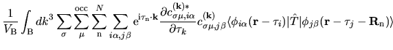
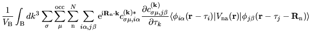
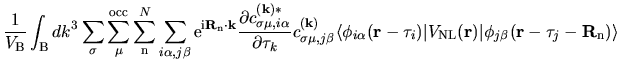
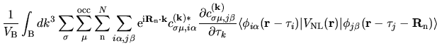
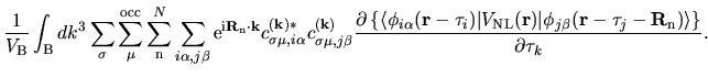
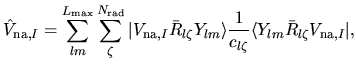
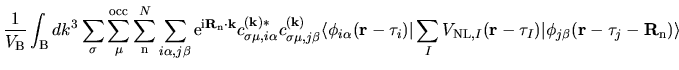
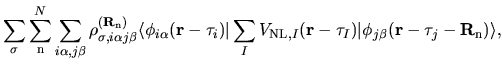
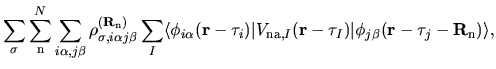
The derivative of the non-local potential energy with respect to
 is given by
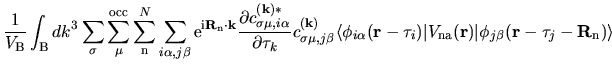
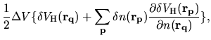
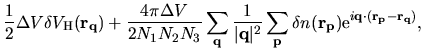
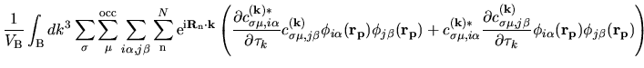
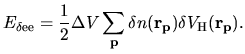
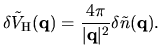
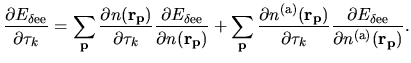
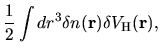
The derivative of the Hartree energy energy for
the difference charge density
 with respect to
  is given by
| |
|
 |
(63) |
Considering Eq. (54) and
| |
|
 |
(64) |
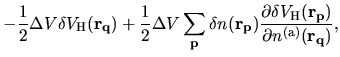
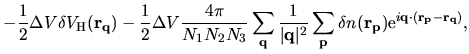
we have
and
Moreover, the derivative of  with respect to
 is given by
The derivative of
 with respect to
 is simply given by
| |
|
 |
(68) |
The derivative of  with respect to the atomic
coordinate
with respect to the atomic
coordinate  is easily evaluated by
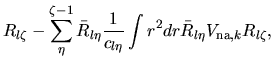
The derivative of the screened core-core Coulomb energy  with respect to
  is given by
| |
|
![$\displaystyle \frac{\partial E_{\rm scc}}{\partial \tau_{k}}
=
\frac{1}{2}\sum_...
...{\bf r})
V^{\rm (a)}_{{\rm H},J}({\bf r})
\right\}
}
{\partial \tau_k}
\right].$](img383.png) |
(70) |
Since the second term is tabulated in a numerical table as a function of
distance due to the spherical symmetry of integrands, the derivative
can be evaluated analytically by employing an
interpolation scheme.
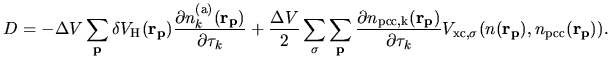
The derivatives given by Eqs. (60), (61), (62), (63), and (69) contain
the derivative of LCPAO coefficient  . The derivative of
  can be
transformed to the derivative of the overlap matrix with respect to
can be
transformed to the derivative of the overlap matrix with respect to
 as shown below.
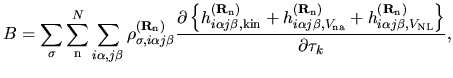
By summing up all the terms including the derivatives of
as shown below.
By summing up all the terms including the derivatives of  in Eqs. (60), (61), (62), (63), and (69), we have
| |
|
 |
(71) |
where  is a diagonal matrix consisting of Heaviside step functions.
Noting that Eq. (27) can be written by
is a diagonal matrix consisting of Heaviside step functions.
Noting that Eq. (27) can be written by
 and
and
 in a matrix form, the product of two diagonal
matrices is commutable, and
in a matrix form, the product of two diagonal
matrices is commutable, and
 for any square matrices,
Eq. (71) can be written as
for any square matrices,
Eq. (71) can be written as
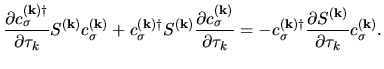
Moreover, taking account of the derivative of the orthogonality
relation
 with respect to
  , we have the following relation:
| |
|
 |
(73) |
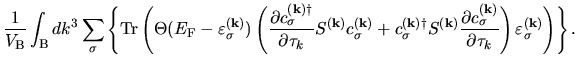
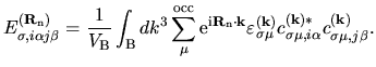
Putting Eq. (73) into Eq. (72), we have
where the energy density matrix
 is given by
| |
|
 |
(74) |
The terms including the derivative of matrix elements
in Eqs. (60), (61), and (62) can be easily evaluated by
| |
|
 |
(75) |
where
The derivatives of these elements are evaluated analytically
from the analytic derivatives of Eqs. (43) and (46).
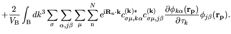
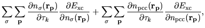
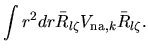
The remaining contributions in first terms of Eqs. (63) and (69)
are given by
| |
|
 |
(79) |
The second terms in Eqs. (63) and (69) becomes
| |
|
 |
(80) |
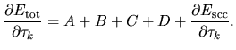
Thus, we see that the derivative of the total energy with
respect to the atomic coordinate  is analytically
evaluated for any grid fineness as
is analytically
evaluated for any grid fineness as
| |
|
 |
(81) |
-
- 1
-
T. Ozaki and H. Kino, Phys. Rev. B 72, 045121 (2005).
- 2
-
T. Ozaki, Phys. Rev. B 67, 155108 (2003).
- 3
-
T. Ozaki and H. Kino, Phys. Rev. B 69, 195113 (2004).
- 4
-
P. E. Blochl, Phys. Rev. B 41, R5414 (1990).
- 5
-
J. M. Soler, E. Artacho, J. D. Gale, A. Garcia, J. Junquera,
P. Ordejon, and D. Sanchez-Portal,
J. Phys.: Condens. Matter 14, 2745 (2002).
2008-11-23


![$\displaystyle +
\frac{1}{2}\sum_{I,J}
\left[
\frac{Z_{I}Z_{J}}
{\vert \tau_{I}-...
...
-
\int dr^3 n^{\rm (a)}_{I}({\bf r})
V^{\rm (a)}_{{\rm H},J}({\bf r})
\right],$](img122.png)
![$\displaystyle +
\frac{1}{2}\sum_{I,J}
\left[
\frac{Z_{I}Z_{J}}
{\vert \tau_{I}-...
...int n^{\rm (a)}_{I}({\bf r})
V^{\rm (a)}_{{\rm H},J}({\bf r})
d{\bf r}
\right],$](img125.png)
![$\displaystyle \frac{1}{2}\sum_{I,J}
\left[
\frac{Z_{I}Z_{J}}
{\vert \tau_{I}-\t...
...
-
\int dr^3 n^{\rm (a)}_{I}({\bf r})
V^{\rm (a)}_{{\rm H},J}({\bf r})
\right].$](img140.png)
![$\displaystyle \left[
\left( \frac{1}{\sqrt{2\pi}} \right )^3
4\pi
(-{\rm i})^{l}
\int dr
r^2
R_{pl}(r)
j_{l}(kr)
\right]
Y_{lm}(\hat{\bf k}),$](img213.png)


![$\displaystyle \sum_{j\beta}
c_{\sigma\mu,j\beta}
\left[
\sum_{{\rm n}}^{N}
{\rm...
...}({\bf r_p})
\delta V_{\rm H}({\bf r}_{\bf p})
\phi_{j\beta}({\bf r_p})
\right]$](img315.png)

![$\displaystyle \sum_{j\beta}
c_{\sigma\mu,j\beta}
\left[
\sum_{{\rm n}}^{N}
{\rm...
...}({\bf r_p})
v_{{\rm xc},\sigma}
({\bf r_p}
)
\phi_{j\beta}({\bf r_p})
\right],$](img320.png)