Analysis of band structures

First, let us analyze how each band can be decomposed into each contribution of pseudo-atomic orbital in a band structure calculation for a primitive cell of SiC in a two-dimensional honeycomb structure without imperfection. Note that unfolding bands is not performed in this case. The SCF calculation for the primitive cell of the two-dimensional SiC can be performed as

  % mpirun -np 16 openmx SiC_Primitive.dat > sic_primitive.std & 

The input file 'SiC_Primitive.dat' can be found in the directory 'work/unfolding_example', and the basis functions and geometrical structure are specified as

  Species.Number       3
  <Definition.of.Atomic.Species
  C    C7.0-s2p2d1     C_PBE13
  Si   Si7.0-s2p2d1    Si_PBE13
  Te  Te11.0-s2p2d2f1  E
  Definition.of.Atomic.Species>

  Atoms.Number    3
  Atoms.SpeciesAndCoordinates.Unit  FRAC  # Ang|AU
  <Atoms.SpeciesAndCoordinates
  1  C    0.33333333   0.66666666   0.50000000   2.0  2.0
  2  Si   0.66666666   0.33333333   0.50000000   2.0  2.0
  3  Te   0.00000000   0.00000000   0.50000000   0.0  0.0
  Atoms.SpeciesAndCoordinates>

  Atoms.UnitVectors.Unit             Ang   # Ang|AU
  <Atoms.UnitVectors
  3.0690  0.0000000000   0.000
  -1.5345  2.6578319641   0.000
  0.0000  0.0000000000  10.000
  Atoms.UnitVectors>

where an empty atom having basis functions with a long tail is allocated at the center of the hexagon in order to improve description of conduction bands. Since the keyword 'Band.dispersion' is switched on as

  Band.dispersion              on       # on|off, default=off
  Band.Nkpath                   3
  <Band.kpath
  60 0.33333333333 0.33333333333 0.00000000000  0.00000000000 0.00000000000 0.00000000000 K G
  52 0.00000000000 0.00000000000 0.00000000000  0.50000000000 0.00000000000 0.00000000000 G M
  30 0.50000000000 0.00000000000 0.00000000000  0.33333333333 0.33333333333 0.00000000000 M K
  Band.kpath>

you might be able to plot the band dispersion using 'sic_primitive.BANDDAT1' as the solid line shown in Fig. 50(a). As for plotting the band dispersion, please refer the section 'Band dispersion'.

Keywords relevant to analysis of band structure

For the calculation, the following keywords are also given as well

  Unfolding.Electronic.Band      on       # on|off, default=off
  Unfolding.LowerBound        -10.0       # default=-10 eV
  Unfolding.UpperBound          6.0       # default= 10 eV

  Unfolding.Nkpoint               4

  <Unfolding.kpoint
  K 0.33333333333 0.33333333333 0.0000000000
  G 0.00000000000 0.00000000000 0.0000000000
  M 0.50000000000 0.00000000000 0.0000000000
  K 0.33333333333 0.33333333333 0.0000000000
  Unfolding.kpoint>

  Unfolding.desired_totalnkpt    30

The specification of the keywords above are listed below.

• Unfolding.Electronic.Band on$\vert$ off, default=off

  To analyze and/or unfold bands the keyword should be switched on. The default is 'off'.

• Unfolding.LowerBound

  The keyword 'Unfolding.LowerBound' specifies the lower bound for the energy of bands in the analysis, where the energy is taken as the relative energy to the chemical potential. The default value is -10 eV.

• Unfolding.UpperBound

  The keyword 'Unfolding.UpperBound' specifies the upper bound for the energy of bands in the analysis, where the energy is taken as the relative energy to the chemical potential. The default value is 10 eV.

• Unfolding.Nkpoint

  The keyword 'Unfolding.Nkpoint' specifies the number of k-points appearing in the keyword 'Unfolding.kpoint'.

• Unfolding.kpoint

  The keyword 'Unfolding.kpoint' specifies the k-points of which number is given by the keyword 'Unfolding.Nkpoint'. In the above case four k-points are given, and three k-paths conecting the two k-points are considered, i.e., one from 'K' to 'G', one from 'G' to 'M', and one from 'M' to 'K'. Along the k-paths the analysis of bands is performed. Note that the unit for the k-points specified by the keyword is the reciprocal lattice vectors of the unit cell given by the keyword 'Atoms.UnitVectors' in this case, while the cell vectors can be changed to perform unfolding of bands by utilizing a keyword 'Unfolding.ReferenceVectors'. At this moment, it should be noted that the reciprocal lattice vectors of the unit cell given by the keyword 'Atoms.UnitVectors' is automatically used unless the keyword 'Unfolding.ReferenceVectors' is explicitly specified. The keyword 'Unfolding.ReferenceVectors' will be explained in the next subsection.

• Unfolding.desired_totalnkpt

  The k-paths specified by the keyword 'Unfolding.kpoint' are divided with a nearly equal spacing, where the spacing is estimated by (the total length of all the k-paths)/Unfolding.desired_totalnkpt. Starting from the estimated spacing, the actual spacing is automatically adjusted from one k-path to another k-path so that the k-points specified by the keyword 'Unfolding.kpoint' can be always included in the analysis.

Output files relevant to analysis of band structure

After getting the SCF convergence, the following files related to analyzing and/or unfolding bands will be generated.

• sic_primitive.unfold_totup

  The total spectral weight given by Eq. (24) in Ref. [98] is stored. The first, second, and third columns correspond to the distance measured from the first k-point given by the keyword 'Unfolding.kpoint' in the unit of Bohr$^{-1}$, energy relative to the chemical potential in the unit of eV, and the total spectral weight, respectively. In the spin-polarized calculation, 'System.Name.unfold_totdn' is also generaged for the down spin case, while only a single file 'System.Name.unfold_tot' is generated in the non-collinear calculation.

• sic_primitive.unfold_orbup

  The orbitally decomposed spectral weights given by Eq. (26) in Ref. [98] are stored. The first, second, and subsequent columns correspond to the distance measured from the first k-point given by the keyword 'Unfolding.kpoint' in the unit of Bohr$^{-1}$, energy relative to the chemical potential in the unit of eV, and the orbitally decomposed spectral weights, respectively. The sequence of the orbitally decomposed spectral weights can be found in 'System.Name.out'. In the spin-polarized calculation, 'System.Name.unfold_orbdn' is also generaged for the down spin case, while only a single file 'System.Name.unfold_orb' is generated in the non-collinear calculation.

• sic_primitive.unfold_plotexample

  As an example of plotting above the data by gnuplot, 'System.Name.unfold_plotexample' is generated. On the command line of the gnuplot, one can perform as

    gnuplot> load `sic_primitive.unfold_plotexample'
  

  
  According to your purpose, it is needless to say that you can modify the file.

  
  

By plotting both 'sic_primitive.BANDDAT1' and 'sic_primitive.unfold_totup' as

  gnuplot> set style data lines
  gnuplot> set zeroaxis
  gnuplot> set key below
  gnuplot> set ytics 1
  gnuplot> set mytics 5
  gnuplot> set xra [0.000000:1.708883]
  gnuplot> set yra [-10.0:6.0]
  gnuplot> set ylabel "eV"
  gnuplot> set xtics ("K" 0.000000, "G" 0.722258, "M" 1.347753, "K" 1.708882)
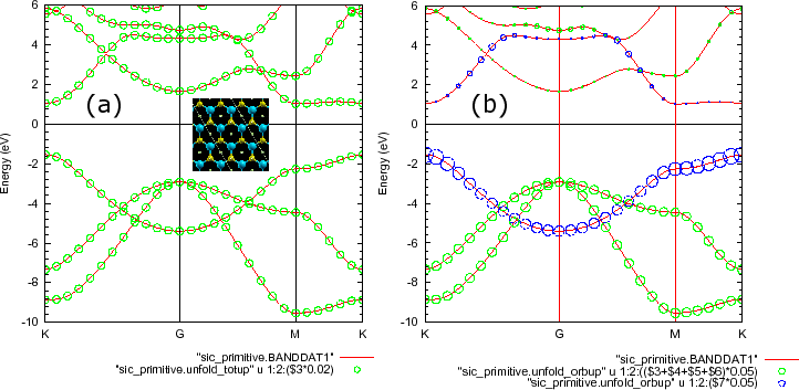
  gnuplot> p "sic_primitive.BANDDAT1","sic_primitive.unfold_totup" u 1:2:($3*0.02) w circle

one may obtain a figure as shown in Fig. 50(a), where the solid line and circle correspond to
"sic_primitive.BANDDAT1" and "sic_primitive.unfold_totup", respectively. The radius of the circle reflects the spectral weight, and all the radii are unity in this case, resulting in the equivalent radius for all the points, since we analyze the band dispersion represented by the Brillouin zone of the original cell.

Now let's move on 'sic_primitive.unfold_orbup' storing orbitally decomposed spectral weights. In a similar way above, one can plot the orbitally decomposed spectral weights as

  gnuplot> p "sic_primitive.BANDDAT1","sic_primitive.unfold_orbup" u 1:2:(($3+$4+$5+$6)*0.05) w circle,
  "sic_primitive.unfold_orbup" u 1:2:($7*0.05) w circle

Then, you may obtain a figure as shown in Fig. 50(b). In this case, the sum of spectral weights for the $s$, $p_x$, and $p_y$ orbitals, and the $p_z$ orbitals on the carbon atom are shown by the green and purple circles, respectively. It can be confirmed from the analysis that the $\sigma$ and $\pi$ bands are clearly distinguished. As for the format of 'sic_primitive.unfold_orbup', please refer the explanation above.

Figure 50: (a) Band structure of SiC primitive cell in a two-dimensional honeycomb structure without imperfection as shown in the inset, where the red line was obtained by the conventional calculation, and the green circles represent the total spectral weight. The radius reflects the magnitude of the weight. (b) Orbitally decomposed spectral weights of SiC primitive cell in a two-dimensional honeycomb structure without imperfection, where the green and purple circles represent the sum of spectral weights for the $s$, $p_x$, and $p_y$ orbitals, and the $p_z$ orbitals on the carbon atom, respectively. The radius reflects the magnitude of the weight. The calculation was performed by using an input file 'SiC_Primitive.dat' in the directory 'work/unfolding_example'.