Next: The origin of the Up: Unfolding method for band Previous: Analysis of band structures Contents Index
In the subsection, we show how the band structure calculated for a supercell can be unfolded
into the Brillouin zone of a reference unit cell that a user specifies.
As an example, let us consider again SiC in a two-dimensional honeycomb structure without imperfection.
However, the unit cell in this case is extended to the (![]() ) supercell as given by
) supercell as given by
  Atoms.Number 12
  Atoms.SpeciesAndCoordinates.Unit  FRAC  # Ang|AU
  <Atoms.SpeciesAndCoordinates
  1 C    0.16666666   0.33333333   0.50000000  2 2
  2 C    0.66666666   0.33333333   0.50000000  2 2
  3 C    0.16666666   0.83333333   0.50000000  2 2
  4 C    0.66666666   0.83333333   0.50000000  2 2
  5 Si   0.33333333   0.16666666   0.50000000  2 2
  6 Si   0.83333333   0.16666666   0.50000000  2 2
  7 Si   0.33333333   0.66666666   0.50000000  2 2
  8 Si   0.83333333   0.66666666   0.50000000  2 2
  9 Te   0.00000000   0.00000000   0.50000000  0 0
  10 Te   0.50000000   0.00000000   0.50000000  0 0
  11 Te   0.00000000   0.50000000   0.50000000  0 0
  12 Te   0.50000000   0.50000000   0.50000000  0 0
  Atoms.SpeciesAndCoordinates>

  Atoms.UnitVectors.Unit             Ang   # Ang|AU
  <Atoms.UnitVectors
  6.138  0.0000000000  0.00
  -3.069  5.3156639282  0.00
  0.000  0.0000000000 10.00
  Atoms.UnitVectors>
% mpirun -np 16 openmx SiC_C_NSP_P.dat > sic_c_nsp_p.std &
  sic_c_nsp_p.unfold_totup
  sic_c_nsp_p.unfold_orbup
  sic_c_nsp_p.unfold_plotexample
To perform the unfolding of bands in the calculation, the following keywords are specified in addition to the keywords explained in the previous subsection:
  <Unfolding.ReferenceVectors
  3.0690  0.0000000000   0.000
  -1.5345  2.6578319641   0.000
  0.0000  0.0000000000  10.000
  Unfolding.ReferenceVectors>

  <Unfolding.Map
  1 1
  2 1
  3 1
  4 1
  5 2
  6 2
  7 2
  8 2
  9 3
  10 3
  11 3
  12 3
  Unfolding.Map>
With the keyword 'Unfolding.ReferenceVectors' one can define a reference unit cell for which the unfolding of bands is performed based on Eq. (24) in Ref. [98]. In the example, the primitive cell was used as the reference cell. The format is the same as that for the keywords 'Atoms.UnitVectors', i.e., the first, second, and third lines correspond to a-, b-, and c-axes, respectively. It is also noted that the unit of the reference unit cell is the same as that used for the supercell, which is specified by the keyword 'Atoms.UnitVectors.Unit'. In the subsection 'Analysis of band structures', the keyword 'Unfolding.ReferenceVectors' was not specified explicitly. In such a case, 'Atoms.UnitVectors' is automatically set for 'Unfolding.ReferenceVectors'.
The keyword 'Unfolding.Map' specifies how atoms in the supercell can be mapped to atoms in the reference cell. The first and second columns are the serial number of atom, which corresponds to the number of the first column in the specification of the keyword 'Atoms.SpeciesAndCoordinates', and an identification number representing the group to which the atom belongs. In the example above, atoms 1 to 4 belong to the group 1, and atoms 5 to 6 the group 2, and atoms 9 to 12 the group 3. Based on the information given by the keyword 'Unfolding.Map', the relabelling of the index for each atom is performed as given by Eq. (17) in Ref. [98], which is the the essential part in the unfolding procedure. It is also noted that the identification number should be positive and integer, while the the integer needs not to start from '1', and not to appear in ascending order.
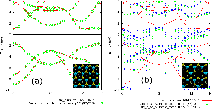
Here we show one more example, i.e., a SiC (![]() ) supercell in a two-dimensional
honeycomb structure with a Si vacancy. The SCF calculation can be performed by
) supercell in a two-dimensional
honeycomb structure with a Si vacancy. The SCF calculation can be performed by
% mpirun -np 16 openmx SiC_C_SP_V.dat > sic_c_sp_v.std &
  Atoms.Number 11
  Atoms.SpeciesAndCoordinates.Unit  FRAC  # Ang|AU
  <Atoms.SpeciesAndCoordinates
  1 C    0.16666666   0.33333333   0.50000000  2.5 1.5
  2 C    0.66666666   0.33333333   0.50000000  2.5 1.5
  3 C    0.16666666   0.83333333   0.50000000  2.5 1.5
  4 C    0.66666666   0.83333333   0.50000000  2.5 1.5
  5 Si   0.33333333   0.16666666   0.50000000  2.5 1.5
  6 Si   0.83333333   0.16666666   0.50000000  2.5 1.5
  7 Si   0.33333333   0.66666666   0.50000000  2.5 1.5
  8 Te   0.00000000   0.00000000   0.50000000  0.0 0.0
  9 Te   0.50000000   0.00000000   0.50000000  0.0 0.0
  10 Te   0.00000000   0.50000000   0.50000000  0.0 0.0
  11 Te   0.50000000   0.50000000   0.50000000  0.0 0.0
  Atoms.SpeciesAndCoordinates>
The mapping of atoms in the supercell to those in the reference cell was specified by
  <Unfolding.Map
  1 1
  2 1
  3 1
  4 1
  5 2
  6 2
  7 2
  8 3
  9 3
  10 3
  11 3
  Unfolding.Map>
After finishing the SCF calculation, you obtain the following files relevant to the unfolding calculation:
  sic_c_sp_v.unfold_totup
  sic_c_sp_v.unfold_totdn
  sic_c_sp_v.unfold_orbup
  sic_c_sp_v.unfold_orbdn
  sic_c_sp_v.unfold_plotexample
When you consider an impurity instead of introduction of vacancy, you only have to assign
the impurity with an identification number. For example, if you introduce an impurity of atom 13
in the SiC (![]() ) supercell, you can define the mapping rule in relabelling as
) supercell, you can define the mapping rule in relabelling as
  <Unfolding.Map
  1 1
  2 1
  3 1
  4 1
  5 2
  6 2
  7 2
  8 2
  9 3
  10 3
  11 3
  12 3
  13 4
  Unfolding.Map>
 |