Mitsuaki Kawamura, ISSP
Date: February 10, 2016
 |
(1) |
 |
(3) |
 |
(4) |
| (6) |
![$\displaystyle {\hat \Gamma}_{\rm L} (\omega) \equiv i \left[ {\hat \Sigma}_{\rm...
...[ {\hat \Sigma}_{\rm R}(\omega) - {\hat \Sigma}^\dagger_{\rm R}(\omega)\right],$](img22.png) |
(7) |
In this section, the Löwdin orthogonalization method is explained; this method is used in the calculations of the Kohn-Sham energy/orbital, the Green's function, the transmission matrix, the eigenchannel, etc. in the non-orthogonal basis representation.
In this section, we obtain the Kohn-Sham equation in the orthogonal basis representation [Eq. (2)] from that equation in the non-orthogonal representation [Eq. (5)].
We decompose the overlap matrix ![]() as
as
| (8) |
| (9) |
The Kohn-Sham equation in the non-orthogonal basis representation [Eq. (5)] becomes
where| (11) |
Comparing Eq. (10) and the Kohn-Sham equation in the orthogonal basis representation [Eq. (2)], we obtain
We can calculate Kohn-Sham orbitals in the non-orthogonal basis representation from those in the orthogonal basis representation as follows:
From (14), we can see
the orthogonal basis ![]() becomes
becomes
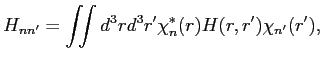
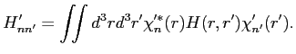
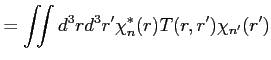
If we have a enough number of orthogonal basis, the transformation from a matrix in the real space representation to that in the orthogonal basis representation
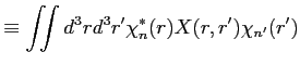 |
(16) |
![$\displaystyle \left[{\hat X}^{-1}\right]_{n n'}$](img40.png) |
![$\displaystyle = \iint d^3 r d^3 r' \chi^{*}_n(r) [X(r,r')]^{-1} \chi_{n'}(r').$](img41.png) |
(17) |
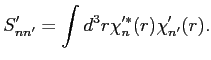
On the other hand, in general, inversion of this matrix in the orthogonal basis space is different from the non-orthogonal basis representation of the inversion of this matrix in the real space:
![$\displaystyle \left[{\hat X}'^{-1}\right]_{n n'} \neq \iint d^3 r d^3 r' \chi'^{*}_n(r) [X(r,r')]^{-1} \chi'_{n'}(r').$](img42.png) |
(18) |
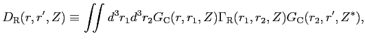
The Green's function of the Kohn-Sham equation in the non-orthogonal basis space [Eq. (5)] is as follows
According to the discussion in the previous section, this Green's function is different from the non-orthogonal basis representation of the Green function of the real-space Kohn-Sham equation, i.e.![$\displaystyle \left[{\hat G}'\right]_{n n'} \neq \iint d^3 r d^3 r' \chi'^{*}_n(r) G(r,r') \chi'_{n'}(r').$](img44.png) |
(20) |
We can obtain the Green's function of the orthogonal basis-space Kohn-Sham equation
[Eq. (2)]
from above
![]() as follows:
as follows:
We can obtain the self energy for the orthogonal basis-space Green's function
from the self energy for
![]()
| (22) |
The device Green's function and linewidths
in the orthogonal basis space (
![]() )
can be obtained by using those calculated from the Hamiltonian in the non-orthogonal basis space
(
)
can be obtained by using those calculated from the Hamiltonian in the non-orthogonal basis space
(
![]() ) as follows:
) as follows:
| (23) | ||
| (24) |
In this section, we obtain the orthogonal basis representation of the transmission matrix
(where| (26) | ||
| (27) |
In this section, we explain the energy normalized eigenchannel proposed
in Ref. [1].
The eigenchannel in the orthogonal basis representation
![]() and the corresponding eigenvalue
and the corresponding eigenvalue ![]() are calculated as follows:
are calculated as follows:
| (28) |
| (29) |
The eigenchannel in the non-orthogonal basis representation
![]() is obtained in the same way to the Kohn-Sham orbital [Eq. (14)];
is obtained in the same way to the Kohn-Sham orbital [Eq. (14)];
| (30) |
| (31) |
Because ![]() is not an Hermite matrix, eigenchannels
is not an Hermite matrix, eigenchannels
![]() are not orthogonal in each other, i.e. even if
are not orthogonal in each other, i.e. even if ![]() ,
,
| (32) |
| (33) |
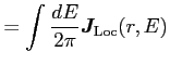
In this section, we explain a method to calculate the current density together with the non-local potential which appears in the Hybrid DFT calculation, non-local pseudopotentials, etc. This method is proposed in Ref. [2]. In this case, we have to consider both the local- and the non-local contributions to the current density as follows [Eqn. (9) in Ref. [2]]:
The first term in Eq. (34) is the local term; this term is calculated as follows [Eqs. (12) and (22) in Ref. [2]]:
 |
(35) | |
| (36) |
 |
(37) |
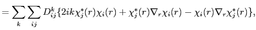
In the orthogonal basis representation,
![]() becomes as follows:
becomes as follows:
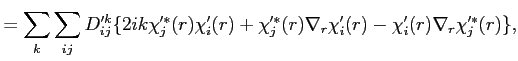
![$\displaystyle D_R(r,r',E)]_{r'=r} = \sum_k [(\nabla_r - \nabla_{r'}) e^{ik(r-r')}\sum_{i j} D_{i j}^k \chi_i(r) \chi_j^*(r')]_{r'=r}$](img114.png) |
||
![$\displaystyle = \left[ \sum_k e^{ik(r-r')}\sum_{i j} D_{i j}^k \chi_j^*(r') (ik + \nabla_{r})\chi_i(r) - \chi_i(r) (-ik + \nabla_{r'})\chi_j^*(r') \right]_{r'=r}$](img115.png) |
||
 |
(38) |
 |
(39) |
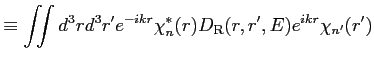
Finally, we can obtain the following non-orthogonal representation by using Eq. (15).
![$\displaystyle = \sum_k \sum_{i j} [{\hat S}_k'^{1/2 \dagger} D' {\hat S}_k'^{1/...
... k [{\hat S}_k'^{-1/2} \chi'^*(r) ]_j [\chi'(r) {\hat S}_k'^{-1/2\dagger}]_i(r)$](img119.png) |
||
![$\displaystyle \hspace{2cm} + [S^{-1/2} \chi'(r)]_j \nabla_{r}[\chi' S^{-1/2\dag...
...r){\hat S}_k'^{-1/2^\dagger}]_i \nabla_{r} [{\hat S}_k'^{-1/2} \chi'^*(r)]_j \}$](img120.png) |
||
 |
(40) |
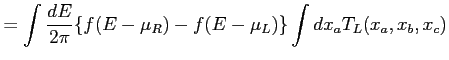
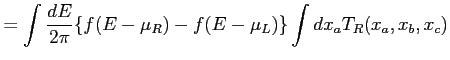
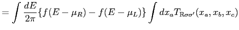
The second term in Eq. (34) is the non-local term; this term is calculated as follows [Eqs. (10) and (11) in Ref. [2]]:
| (41) | ||
| (42) |
 |
(43) | |
![$\displaystyle = i \int d^3r' 2 i {\rm Im}[V(r,r') D(r',r)] [f(E-\mu_R) - f((E-\mu_L)]$](img131.png) |
(44) | |
![$\displaystyle = \sum_k \sum_{i j} [V^k D^k]_{i j} \chi_i(r) \chi_j^*(r)$](img133.png) |
||
![$\displaystyle = \sum_k \sum_{i j} [{\hat S}_k'^{-1/2\dagger} V'^k D'^k {\hat S}...
..._{i j} [\chi'(r) {\hat S}_k'^{-1/2\dagger}]_i [{\hat S}_k'^{-1/2} \chi'^*(r)]_j$](img134.png) |
||
![$\displaystyle = \sum_k \sum_{i j} [{\hat S}_k'^{-1} V'^k D'^k]_{i j} \chi'_i(r) \chi'^*_j(r),$](img135.png) |
(45) |
 |
(46) |
 |
(47) |
The Poisson equation (42) is solved under the following boundary conditions:
| (48) | ||
| (49) |
From the Eq. (34), we obtain
| (50) | ||
| (51) |
 |
(52) | |
$](img155.png) |
||
![$\displaystyle = \sum_k \sum_{i j} \chi_i(r) [G_{{\rm C} k} \Gamma_{{\rm R} k} G_{{\rm C} k}^\dagger \Gamma_{{\rm L} k}]_{i j} \chi^*_j(r)$](img156.png) |
||
![$\displaystyle = \sum_k \sum_{i j} [\chi'(r) {\hat S}_k'^{-1/2\dagger}]_i [{\hat...
... \Gamma'_{{\rm L} k}{\hat S}_k'^{-1/2}]_{i j} [{\hat S}_k'^{-1/2} \chi'^*(r)]_j$](img157.png) |
||
![$\displaystyle = \sum_k \sum_{i j} \chi'_i(r) [G'_{{\rm C} k} \Gamma'_{{\rm R} k} G'^\dagger_{{\rm C} k} \Gamma'_{{\rm L} k} {\hat S}_k'^{-1}]_{i j} \chi'^*_j(r)$](img158.png) |
(53) |
 |
(54) | |
$](img162.png) |
||
![$\displaystyle = \sum_k \sum_{i j} \chi'_i(r) [G'_{{\rm C} k} \Gamma'_{{\rm L} k} G'^\dagger_{{\rm C} k} \Gamma'_{{\rm R} k} {\hat S}_k'^{-1}]_{i j} \chi'^*_j(r)$](img163.png) |
(55) |
We can calculate the spin/charge current density
together with a collinear magnetism.
In this case, first we calculate separately contributions to
![]() in Eq. (34)
from each spin (
in Eq. (34)
from each spin (![]() and
and
![]() )
)
| (56) |
| (57) | ||
| (58) |
In these calculations, we can use the following ![]() -inversion symmetries:
-inversion symmetries:
| (59) | ||
| (60) | ||
| (61) | ||
| (62) |
When we consider the non-collinear magnetization,
we calculate the diagonal and the off-diagonal part
![]() as follows:
as follows:
| (63) | ||
![$\displaystyle = \sum_k \sum_{i j} \int \frac{d E}{2 \pi} [f(E-\mu_L) - f(E-\mu_R)] i D'^k_{i \sigma j \sigma'}$](img185.png) |
||
| (64) | ||
| (65) | ||
| (66) | ||
![$\displaystyle = \int \frac{dE}{2\pi} i \sum_k \sum_{\sigma_1} \int d^3r' [f(E-\mu_R) - f(E-\mu_L)]$](img192.png) |
||
![$\displaystyle = \int \frac{dE}{2\pi} i \sum_k [f(E-\mu_R) - f(E-\mu_L)]$](img194.png) |
||
![$\displaystyle \hspace{1cm} \times \left\{ \sum_{i j} [{\hat S}_k'^{-1} {\hat V}...
...\hat V}'^k {\hat D}'^k]^*_{i \sigma' j \sigma} \chi'^*_i(r) \chi'_j(r) \right\}$](img195.png) |
||
![$\displaystyle = \sum_{i j} [f(E-\mu_R) - f(E-\mu_L)] \chi'_i(r) \chi'^*_j(r)$](img196.png) |
||
![$\displaystyle \hspace{1cm} \times \int \frac{dE}{2\pi} i \sum_k \left\{[{\hat S...
...- [{\hat S}_k'^{-1} {\hat V}'^k {\hat D}'^k]^*_{j \sigma' i \sigma} \right\} %
$](img197.png) |
(67) |
The Poisson equation for
![]() is written as follows:
is written as follows:
| (68) | ||
 |
(69) | |
![$\displaystyle \equiv \sum_k [{\hat G}_{{\rm C} k} {\hat \Gamma}_{{\rm R} k} {\h...
... {\hat \Gamma}'_{{\rm L} k} {\hat S}_k'^{-1}]_{i \sigma j \sigma'} \chi'^*_j(r)$](img204.png) |
(70) | |
 |
(71) | |
![$\displaystyle = \sum_k \sum_{i j} \chi'_i(r) [{\hat G}'_{{\rm C} k} {\hat \Gamm...
... {\hat \Gamma}'_{{\rm R} k} {\hat S}_k'^{-1}]_{i \sigma j \sigma'} \chi'^*_j(r)$](img208.png) |
(72) |
These calculations are performed as that represented in Fig. 1.
We explain functions in the call graph (Fig. 2) as follows:
Set the first index of each atoms in the basis space.
void TRAN_Calc_Diagonalize(int n, dcomplex evec[n*n], double eval[n],
int lscale)
Diagonalize matrix evec and replace it with its eigenvectors.
If lscale=1, eigenvectors are scaled by a fuctor sqrt(eval[i]).
int TRAN_Calc_OrtSpace(int NUM_c, dcomplex SCC[NUM_c * NUM_c],
dcomplex rtS[NUM_c * NUM_c], dcomplex rtSinv[NUM_c * NUM_c])
Compute
![]() (
(rtS) and
![]() (
(rtSinv)
from ![]() (
(SCC). This function returns the number of the orthogonal basis;
it becomes smaller that the number of the non-orthogonal basis(NUM_c).
void TRAN_Calc_Linewidth(int NUM_c, dcomplex SigmaL_R[NUM_c * NUM_c], dcomplex SigmaR_R[NUM_c * NUM_c])
Compute
![]() .
.
void TRAN_Calc_MatTrans(int NUM_c, dcomplex SigmaL_R[NUM_c * NUM_c], dcomplex GC_R[NUM_c * NUM_c], char* trans1, char* trans2)
Compute
![]() .
.
void TRAN_Calc_LowdinOrt(
int NUM_c, dcomplex SigmaL_R[NUM_c * NUM_c], dcomplex SigmaR_R[NUM_c * NUM_c],
int NUM_cs, dcomplex rtS[NUM_c * NUM_c], dcomplex rtSinv[NUM_c * NUM_c],
dcomplex ALbar[NUM_cs * NUM_cs], dcomplex GamRbar[NUM_cs * NUM_cs])
Perform the Löwdin orthogonalization of
![]() and
and
![]() .
.
void TRAN_Calc_ChannelLCAO(int NUM_c, int NUM_cs,
dcomplex rtSinv[NUM_c * NUM_c], dcomplex ALbar[NUM_cs * NUM_cs],
dcomplex GamRbar[NUM_cs * NUM_cs], double eval[NUM_cs],
dcomplex GC_R[NUM_c * NUM_c], int TRAN_Channel_Num,
dcomplex EChannel[TRAN_Channel_Num][NUM_c],
double eigentrans[TRAN_Channel_Num])
Transform Eigenchannel in the orthogonalized basis space into that in the non-orthogonalized basis space.
static void Print_CubeTitle_EigenChannel(
FILE *fp,
double TRAN_Channel_kpoint[2],
double TRAN_Channel_energy,
double eigentrans,
int ispin)
static void Print_CubeTitle_EigenChannel_Bin(
FILE *fp,
double TRAN_Channel_kpoint[2],
double TRAN_Channel_energy,
double eigentrans,
int ispin)
Output the comment, atomic positions, the number of grid, and the grid offset
to a .cube or a .cube.bin file.
void TRAN_Output_ChannelLCAO(
int myid0,
int kloop,
int iw,
int ispin,
int NUM_c,
double TRAN_Channel_kpoint[2],
double TRAN_Channel_energy,
double eval[NUM_c],
dcomplex GC_R[NUM_c * NUM_c],
double eigentrans_sum[TRAN_Channel_Nenergy][SpinP_switch+1])
Output eigenchannels as a LCAO coefficient.
TRAN_Output_ChannelCube(
int kloop,
int iw,
int ispin,
int orbit,
int NUM_c,
double *TRAN_Channel_kpoint,
dcomplex EChannel[NUM_c],
int MP[atomnum],
double eigentrans,
double TRAN_Channel_energy)
Output eigenchannels as a real-space .cube format.
void TRAN_Output_eigentrans_sum(
int TRAN_Channel_Nkpoint,
int TRAN_Channel_Nenergy,
double eigentrans_sum[TRAN_Channel_Nkpoint][TRAN_Channel_Nenergy])
Output the sum of transmission eigenvalues in each ![]() and energy.
and energy.
void TRAN_Calc_Sinv(
int NUM_c,
dcomplex SCC[NUM_c * NUM_c],
dcomplex Sinv[NUM_c * NUM_c])
Compute
![]() .
.
void TRAN_Calc_CurrentDensity(
int NUM_c,
dcomplex GC[NUM_c * NUM_c],
dcomplex GammaL[NUM_c * NUM_c],
dcomplex GammaR[NUM_c * NUM_c],
dcomplex VCC[NUM_c * NUM_c],
dcomplex Sinv[NUM_c * NUM_c],
double kvec[2],
double fL,
double fR,
double Tran_current_energy_step,
double JLocSym[2][NUM_c][NUM_c],
double JLocAsym[NUM_c][NUM_c],
double RhoNL[NUM_c][NUM_c],
double Jmat[2]
)
void TRAN_Calc_CurrentDensity_NC(
int NUM_c,
dcomplex GC[NUM_c * NUM_c],
dcomplex GammaL[NUM_c * NUM_c],
dcomplex GammaR[NUM_c * NUM_c],
dcomplex VCC[NUM_c * NUM_c],
dcomplex Sinv[NUM_c * NUM_c],
double kvec[2],
double fL,
double fR,
double Tran_current_energy_step,
double JLocSym[4][2][NUM_c * NUM_c],
double JLocAsym4[4][NUM_c * NUM_c],
double RhoNL[4][NUM_c * NUM_c],
double Jmat[4][2][NUM_c * NUM_c]
)
Compute the contribution from each ![]() , energy component to the currentdensity.
, energy component to the currentdensity.
static double TRAN_Calc_Orb2Real(
int NUM_c, int MP[atomnum],
double JOrb[NUM_c][NUM_c], double JReal[TNumGrid],
dcomplex SCC[NUM_c * NUM_c])
Compute
![]() .
.
static void TRAN_Current_dOrb(int NUM_c, int *MP, double JSym[2][NUM_c][NUM_c], double JASym[NUM_c][NUM_c], double JReal[3][TNumGrid])
Compute
![]() .
.
static void TRAN_Integrate1D(double Jmat[2][TNumGrid],
dcomplex Jbound[2][Ngrid2*Ngrid3], double Current[TNumGrid])
Compute partial trace for ![]() for the boundary current.
for the boundary current.
static void TRAN_Current_Boundary(dcomplex JBound[2][Ngrid2*Ngrid3])
Perform the Fourier transform of the boundary current.
static void FFT2D_CurrentDensity(double ReRhok[My_Max_NumGridB],
double ImRhok[My_Max_NumGridB])
Perform 2D-FFT of
![]() into the reciplocal space.
into the reciplocal space.
static void TRAN_Poisson_Current(double Rho[TNumGrid],
dcomplex Jbound[2][Ngrid2*Ngrid3])
Solve the Poisson equation for
![]() .
.
static void TRAN_Current_AddNLoc(double Rho[TNumGrid],
double Current[3][TNumGrid])
Sum the local- and non-local part of the currentdensity.
static void TRAN_Current_Spin(double CDensity[SpinP_switch + 1][3][TNumGrid])
Compute the charge- and the spin currentdensities from the each spin components of the currentdensity.
static void TRAN_Voronoi_CDEN(double CDensity[SpinP_switch + 1][3][TNumGrid], int TRAN_OffDiagonalCurrent)
Perform the Voronoianalysis of the currentdensity and output it.
![$\displaystyle \chi_n(r) = \sum_{n'}\chi'_{n'}(r)[{\hat S}'^{-1/2 \dagger}]_{n' n}.$](img37.png)

![\includegraphics[width=15cm]{flow.eps}](img209.png)
![\includegraphics[width=15cm]{call_graph.eps}](img210.png)